This introduction fine-tunes your COMSOL Multiphysics® modeling skills for heat transfer simulations. The model tutorial solves a conjugate heat transfer problem from the field of electronic cooling, but the principles are applicable to any field involving heat transfer in solids and fluids.
Conduction is a form of heat transfer that can be described as proportional to the temperature gradients in a system. This is formulated mathematically by Fourier’s law. The Heat Transfer Module describes conduction in systems where thermal conductivity is constant or is a function of temperature or any other model variable, for example, chemical composition.
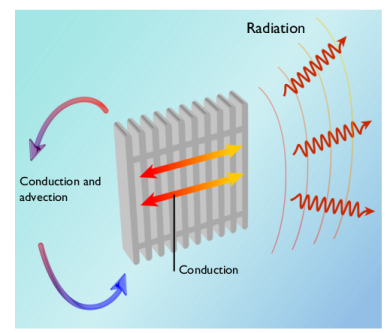
In the case of a moving fluid, the energy transported by the fluid has to be modeled in combination with fluid flow. This is referred to as convection of heat and must be accounted for in forced and free convection (conduction and advection). This module includes descriptions for heat transfer in fluids and conjugate heat transfer (heat transfer in solids and fluids in the same system), for both laminar and turbulent flows. In the case of turbulent flow, the module offers two algebraic turbulence models, the
Algebraic yPlus and
L-VEL models, as well as the standard
k-ε model for high-Reynolds numbers, the low Reynolds number
k-ε model, and the SST (shear stress transport) model to accurately describe conjugate heat transfer. The Gravity feature defines buoyancy forces induced by density differences, in particular due to temperature dependency of the density.
Radiation is the third mechanism for heat transfer that is included in the module. The associated features handle surface-to-ambient radiation, surface-to-surface radiation, and external radiation sources (for example, the sun). The surface-to-surface radiation capabilities support mixed diffuse-specular reflection as well as transmission through semitransparent layers. Surface properties may be a function of several parameters, in particular of the position, the temperature, the wavelength or the incident angle. The Heat Transfer Module also contains functionality for radiation in participating and absorbing media. This radiation model accounts for the absorption, emission, and scattering of radiation by the material present between radiating surfaces. The module offers three models for participating and absorbing media simulations: the discrete ordinates method (DOM), the P1 method, and the Rosseland approximation. Finally the Radiative Beam in Absorbing Media interface provides features to define the absorbing media properties, as well as options for multiple incident beams.
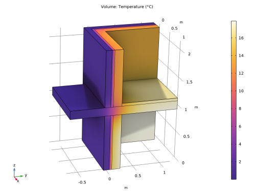
The Building and Constructions section in the Application Library includes files that are related to energy efficiency and dissipation in buildings. Most of these use convective heat flux to account for heat exchange between a structure and its surroundings. Simulation provides accurate depictions of the heat and energy fluxes that inform energy management in buildings and construction.
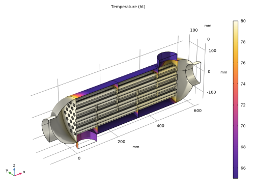
The Heat Exchangers section in the Application Library presents several heat exchangers of different sizes, flow arrangements, and flow regimes. They benefit from the predefined Conjugate Heat Transfer interface that provides ready-to-use features for couplings between solids, shells, and laminar or turbulent flows. The simulation results show properties of the heat exchangers, such as their efficiency, pressure loss, or compactness.
The Medical Technology section in the Application Library introduces the concept of bioheating. Here, the influences of various processes in living tissue are accounted for as contributions to heat flux and as sources and sinks in the heat balance relations. Bioheating applications that can be modeled include the microwave heating of tumors (such as hyperthermia cancer therapy) and the interaction between microwave antennas and living tissue (such as the influence of a diagnostic probe or cellphone use on the temperature of tissue close to the ear). The benefit of using the bioheat equation is that it has been validated for different types of living tissue, using empirical data for the different properties, sources, and sinks. In addition, damage-integral features are provided to model tissue necrosis due to hyperthermia or hypothermia. The models and simulations available in this physics interface provide excellent complements to experimental and clinical trials; the results may be used for many purposes, for example, to develop new methods for dose planning.
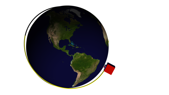
The Orbital Thermal Loads section in the Application Library presents applications related to spacecraft thermal analysis. All the applications include the definition of the planet, orbit, and spacecraft properties. From this information the position and orientation of the spacecraft, but also the direct solar radiation, albedo, and planet radiative flux as well as the radiative heat transfer between the different spacecraft parts are computed. It is possible to analyze further the heat transfer in the spacecraft by including a heat transfer physics interface in the model to account for the energy balance including the heat conduction in solid parts.
The Phase Change section in the Application Library presents applications such as metal melting, evaporation, and food cooking. A common characteristic of these models is that the temperature field defines the material phase, which has a significant impact on the material properties. Equations representing the highly nonlinear behavior of the material properties as a function of temperature are automatically generated by the Phase Change Material subfeature or the Phase Change Interface boundary condition. The phase change model provides information to control material transformation.
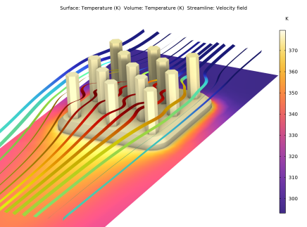
The Power Electronics and Electronic Cooling section in the Application Library includes examples that often involve heat generation, heat transfer in solids, and conjugate heat transfer (where cooling is described in greater detail). The examples in these applications are often used to design cooling systems and to control the operating conditions of electronic devices and power systems. The module provides the tools needed to understand and optimize flow and heat transfer mechanisms in these systems when the model results are interpreted.

The Thermal Contact and Friction section in the Application Library contains examples where thermal cooling is dependent on a thermal contact or where the heat source is due to friction. The thermal contact properties can be coupled with structural mechanics that provide the contact pressure at the interface. It is also possible to combine thermal contact and electrical contact in the same model.
The Thermal Processing section in the Application Library contains examples that include thermal processes, such as continuous casting. A common characteristic of most of these examples is that the temperature field and the temperature variations have a significant impact on the material properties or the physical behavior (thermal expansion, thermophoresis, and so forth) of the modeled process or device. Since these couplings make the processes very complicated, modeling and simulation often provide a useful shortcut to a complex understanding.
The Thermal Radiation section in the Application Library contains applications where heat transfer by radiation must be considered in order to describe the heat flux accurately. A common feature of these examples is that they contain devices where high radiative heat transfer is observed due to high temperature, high surface emissivity, or external radiation like solar radiation. These applications account for the nonlinearity that results from the radiative heat transfer and geometric effects such as shielding between two radiating objects. The geometry or the radiation source may be moving or deformed during the simulation.
The Thermal Stress section in the Application Library presents examples where the temperature field causes thermal expansion. Thermal stress can result from heat exchanges between cold and hot devices or from processes like Joule heating. These require the Structural Mechanics Module or the MEMS Module for the portions where structural mechanics are simulated.
The Tutorials section in the Application Library contains examples that demonstrate the implementation of a particular phenomenon or the use of some features. Reproducing these applications is an effective method to discover the capabilities of the Heat Transfer Module and to get more experience using it.
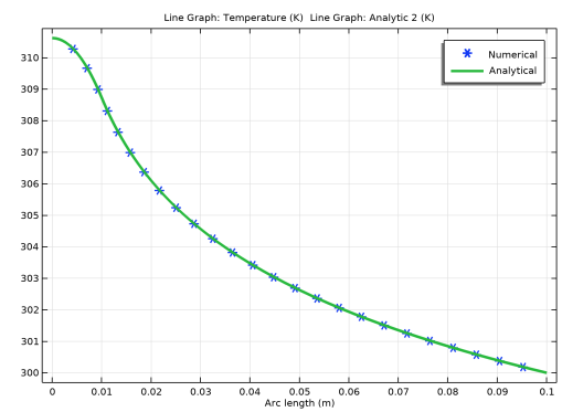
The Verification Examples section in the Application Library provides examples that reproduce a case with a known solution and compare it with COMSOL Multiphysics results.