This section contains information about the available shape function types (element types). See also Elements and Shape Function Programming in the COMSOL Multiphysics Programming Reference Manual.

The preceding examples are special cases of the Lagrange element. Consider a positive integer k, the order of the Lagrange element. For simplex mesh elements, the functions u in this finite element space are piecewise polynomials of degree k; that is, on each mesh element u is a polynomial of degree k. Also, in the following table, l, m, and n are nonnegative integers. In general, for a mesh element of type T, u belongs to the Lagrange shape function space Lagk(T), which is spanned by the following monomials (or rational functions, in the case of pyramid elements):

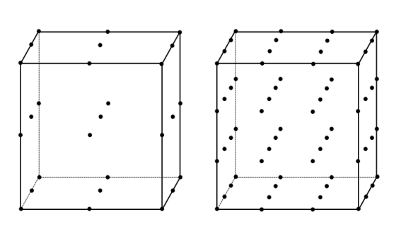
To describe such a function it suffices to give its values in the Lagrange points of order k. These are the points whose local (element) coordinates are integer multiples of 1/k. For example, for a triangular mesh in 2D with k = 2, this means that you have node points at the corners and side midpoints of all mesh triangles. For each of these node points pi, there exists a degree of freedom Ui = u(pi) and a basis function φi. The restriction of the basis function φi to a mesh element is a function in Lagk(T) such that φi = 1 at node i, and φi = 0 at all other nodes. The basis functions are continuous and you have

The Lagrange elements are available with all types of mesh elements, and it is the most common element type in the physics interfaces. The order k can be arbitrary, but the available numerical integration formulas usually limits its usefulness to k ≤ 5(k ≤ 4 for tetrahedral meshes).

For order k = 1, the Lagrange shape space has dimension 2 and has the following basis:

For order k = 2 the Lagrange shape space has dimension 3 and has the following basis:

For order k = 1, the Lagrange shape space has dimension 3 and has the following basis:

For order k = 2, the Lagrange shape space has dimension 6 and has the following basis:

For order k = 1, the Lagrange shape space has dimension 4 and has the following basis:

For order k = 2, the Lagrange shape space has dimension 9 and has the following basis:

For order k = 1, the Lagrange shape space has dimension 4 and has the following basis:

For order k = 2, the Lagrange shape space has dimension 10 and has the following basis:

For order k = 1, the Lagrange shape space has dimension 8 and has the following basis:

The Lagrange element defines the following variables. Denote basename with u, and let x and y denote (not necessarily distinct) spatial coordinates. The variables are (sdim = space dimension and edim = mesh element dimension):

When calculating the derivatives, the global spatial coordinates are expressed as polynomials of degree (at most) sorder in the local coordinates.

On each mesh element, the functions in the nodal serendipity finite element space is a subset of those of the Lagrange element. For simplex mesh elements, the functions u in this finite element space are piecewise polynomials of degree k, where k = 2, 3, or 4; that is, on each mesh element u is a polynomial of degree k. In the following table, l, m, and n are nonnegative integers. Also, define a function sl(i) (for the superlinear order) such that sl(i) is equal to i, if i > 1; else sl(i) = 0. In general, for a mesh element of type T, u belongs to the nodal serendipity shape function space Serk(T), which is spanned by the following monomials (or rational functions, in the case of pyramid elements):

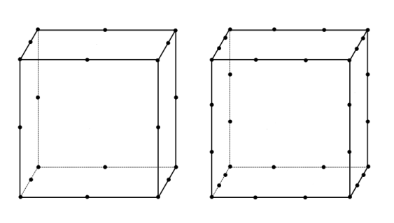
To describe such a function it suffices to give its values in the serendipity points of order k, where k is 2, 3, or 4. These points are a subset of the Lagrange points (see The Lagrange Element). For each of these node points pi, there exists a degree of freedom Ui = u(pi) and a basis function φi. The restriction of the basis function φi to a mesh element is a function in Lagk(T) such that φi = 1 at node i, and φi = 0 at all other nodes. The basis functions are continuous and you have

The nodal serendipity element defines the following field variables. Denote basename with u, and let x and y denote (not necessarily distinct) spatial coordinates. The variables are (sdim = space dimension and edim = mesh element dimension):

When calculating the derivatives, the global spatial coordinates are expressed as polynomials of degree (at most) sorder in the local coordinates.

For a function represented with Lagrange elements, the first derivatives between mesh elements can be discontinuous. In certain equations (for example, the biharmonic equation) this can be a problem. The Argyris element has basis functions with continuous derivatives between mesh triangles (it is defined in 2D only). The second-order derivative is continuous in the triangle corners. On each triangle, a function u in the Argyris finite element space is a polynomial of degree 5 in the local coordinates.

The Argyris element defines the following degrees of freedom (where u is the base name and x and y are the spatial coordinate names):

The Argyris element defines the following field variables (where sdim = space dimension = 2 and edim = mesh element dimension):

On each mesh element, the functions in the Hermite finite element space are the same as for the Lagrange element, namely, all polynomials of degree (at most) k in the local coordinates. The difference lies in which DOFs are used. For the Hermite element, a DOF u exists at each Lagrange point of order k, except at those points adjacent to a corner of the mesh element. These DOFs are the values of the function. In addition, other DOFs exist for the first derivatives of the function (with respect to the global coordinates) at the corners (ux and uy in 2D). Together, these DOFs determine the polynomials completely. The functions in the Hermite finite element space have continuous derivatives between mesh elements at the mesh vertices. However, at other common points for two mesh elements, these derivatives are not continuous. You can think of the Hermite element as lying between the Lagrange and Argyris elements.

The Hermite element is available with all types of mesh elements except pyramids. The order k ≥ 3 can be arbitrary, but the available numerical integration formulas usually limits its usefulness to k ≤ 5 (k ≤ 4 for tetrahedral meshes).

When setting Dirichlet boundary conditions on a variable that has Hermite shape functions, a locking effect can occur if the boundary is curved and the constraint order cporder is the same as the order of the Hermite element. This means that the derivative becomes overconstrained at mesh vertices at the boundary, due to the implementation of the boundary conditions. To prevent this locking, you can specify cporder to be the element order minus 1.

The Hermite element defines the following field variables. Denote basename with u, and let x and y denote (not necessarily distinct) spatial coordinates. The variables are (sdim = space dimension and edim = mesh element dimension):

When calculating the derivatives, the global spatial coordinates are expressed as polynomials of degree (at most) sorder in the local coordinates.

The bubble element has a single degree of freedom, basename, at the midpoint of the mesh element.

The bubble element defines the following field variables. Denote basename with u, and let x and y denote (not necessarily distinct) spatial coordinates. The variables are (sdim = space dimension and edim = mesh element dimension):

In electromagnetics, curl elements (also called vector elements or Nédélec’s elements of the first kind) are widely used. Each mesh element has DOFs corresponding only to tangential components of the field. For example, in a tetrahedral mesh in 3D each of the three edges in a triangle face element has degrees of freedom that are tangential components of the vector field in the direction of the corresponding edges, and in the interior of the triangle there are degrees of freedom that correspond to vectors tangential to the triangle itself (if the element order is high enough). Finally, in the interior of the mesh tetrahedron there are degrees of freedom in all coordinate directions (if the element order is high enough). This implies that tangential components of the vector field are continuous across element boundaries, but the normal component is not necessarily continuous. This also implies that the curl of the vector field is an integrable function, so these elements are suitable for equations using the curl of the vector field.

The precise relation between the vector field (actually a one-form) and the DOFs of the curl element is rather complicated. We start by introducing for every mesh element T of dimension d the local vector shape function space Curlk(T) consisting of vector fields Φ = (Φ1, …, Φd) satisfying the following condition:

where Lagk(T) is the Lagrange shape function space defined in the section on Lagrange shape functions. There is one exception; for pyramid mesh elements the definition needs to be modified as follows:

Next we introduce a transformation between local and global coordinates for a vector field in a mesh element T of dimension d embedded in space of dimension D. For a vector field in global coordinates φ = (φ1, …, φD), the corresponding vector field in local coordinates is Φ = (Φ1, …, Φd) with components defined by

For mesh elements of full dimension d = D, this relation can be inverted to give

In particular, if T has full dimension, is a face or edge of T, and Φ is a vector field on T in local coordinates, then a vector field φ can be computed, and from its restriction to a vector field in local coordinates on .

Only the components of the global coordinate vector field φ can be directly evaluated as variables.

The relation between DOFs and vector fields is defined by specifying in each mesh element a number of pairs (p, v), where p is a point in the mesh element (given in local coordinates) and v is a vector. The DOFs are then defined as

If the number of pairs in each mesh element of type T is chosen to be equal to the dimension of Curlk(T), the values of these DOFs uniquely define the vector field Φ. Typically, some of the pairs (p, v) have p in the interior of T, while others have p on some face or edge . It is convenient to think of the DOFs corresponding to the latter points as inherited from .

Since there might be more than one DOF in the same point p, DOF names have a suffix consisting of two integers, to distinguish different DOFs at the same point.

The choice of pairs (p, v) must take into account the orientation of each mesh element. Failing to do this would result in a vector field whose tangential component changes direction at the boundary between mesh elements. This is done by means of a global numbering of all mesh vertices.

Each edge mesh element has k DOFs. Let P0, P1 be the local coordinates of the endpoints of the edge, written in order of increasing mesh vertex indices (so P0, P1 is some permutation of the points 0 and 1 on the real line). Let v1 be the 1-dimensional vector . In local coordinates, the DOFs on the edge element are defined by the following pairs (p, v):

Each triangular mesh element has k DOFs on each edge (inherited from the corresponding edge elements) and k(k − 1) DOFs in the interior. Let P0, P1, P2 be the local coordinates of the triangle vertices, in order of increasing mesh vertex indices (so P0, P1, P2 is some permutation of the points (0, 0), (1, 0), (0, 1)). Let and . Then the interior DOFs in this triangle are defined by the following pairs (p, v):

Each quadrilateral mesh element has k DOFs on each edge (inherited from the corresponding edge elements) and 2k(k − 1) DOFs in the interior. Let P0 be the local coordinate of the vertex with lowest global index, P1 the other vertex on the same horizontal edge as P0, and P2 the other vertex on the same vertical edge as P0 (so P0, P1, P2 is some subset of the points (0, 0), (1, 0), (0, 1), (1, 1)). Let and . Then the interior DOFs in this quadrilateral are defined by the following pairs (p, v):

Each tetrahedral mesh element has k DOFs on each edge, k(k − 1) DOFs on each face, and k(k − 1)(k − 2)/2 DOFs in the interior. Let P0, P1, P2, P3 be the local coordinates of the tetrahedron vertices, in order of increasing mesh vertex indices (so P0, P1, P2, P3 is some permutation of the points (0, 0, 0), (1, 0, 0), (0, 1, 0), (0, 0, 1)). Let

Then the interior DOFs in this tetrahedron are defined by the following pairs (p, v):

Each hexahedral mesh element has k DOFs on each edge, 2k(k − 1) DOFs on each face, and 3k(k − 1)2 DOFs in the interior. Let P0 be the local coordinate of the vertex with lowest global index, and let P1, P2, P3 be the other vertices that differ from P0 only in the ξ1, ξ2, ξ3 coordinates respectively. Let

Then the interior DOFs in this hexahedron are defined by the following pairs (p, v):

Each prism mesh element has k DOFs on each edge, k(k − 1) DOFs on each triangular face, 2k(k − 1) DOFs on each quadrilateral face, and k(k − 1)(3k − 4)/2 DOFs in the interior. Let P0 be the local coordinate of the vertex with lowest global index, let P1, P2 be the other two vertices on the same triangular face as P0, numbered so that P1 has lower index than P2, and let P3 be the third point connected to P0 by an edge. Let

Then the interior DOFs in this prism are defined by the following pairs (p, v):

Each pyramid mesh element has k DOFs on each edge, k(k − 1) DOFs on each triangular face, 2k(k − 1) DOFs on the quadrilateral face, and k(k − 1)(2k − 1)/2 DOFs in the interior. Let v1 = (1, 0, 0), v2 = (0, 1, 0), and v3 = (0, 0, 1). Then the interior DOFs in this pyramid are defined by the following pairs (p, v):

For convenience we provide here explicit formulas for the Curl shape functions for the lowest orders and most common mesh elements. For each element type, the shape function corresponding to each DOF is written out in local coordinates, for a particular ordering of the mesh element vertices. For other numbers, the difference is that the vector v changes direction for some of the DOFs. For DOFs with suffix 10 this simply means that the corresponding shape functions change sign. Other shape functions might be replaced by a linear combination of the shape functions corresponding to DOFs at the same node point.

For order k = 1, the Curl shape space has dimension 3, and has the following basis:

For order k = 2, the Curl shape space has dimension 8, and has the following basis:

For order k = 1 the Curl shape space has dimension 4, and has the following basis:

For order k = 2 the Curl shape space has dimension 12, and has the following basis:

For order k = 1 the Curl shape space has dimension 6, and has the following basis:

For order k = 1 the Curl shape space has dimension 12, and has the following basis:

The curl element defines the following degrees of freedom: dofbasename d c, where d  =  1 for DOFs in the interior of an edge, d  =  2 for DOFs in the interior of a surface, and so forth, and c is a number between 0 and d  − 1.

The curl element defines the following field variables (where comp is a component name from compnames, and dcomp is a component from dcompnames, sdim = space dimension and edim = mesh element dimension):

For performance reasons, use dcomp in expressions involving the curl rather than writing it as the difference of two gradient components.

For the computation of components, the global spatial coordinates are expressed as polynomials of degree (at most) sorder in the local coordinates.

The curl type 2 element (also called Nédélec’s elements of the second kind) is similar to the curl element that has DOFs corresponding to tangential components of the field. The main difference is that the curl type 2 element has full polynomial orders in all directions for each field component. The theory of curl type 2 elements is introduced in Ref. 1 and Ref. 2.

The functions in the discontinuous Lagrange elements space are the same as for the standard Lagrange element, with the difference that the basis functions are discontinuous between the mesh elements. These elements are available in two variants: discontinuous Lagrange elements and nodal discontinuous Lagrange elements. The difference between these two is that the latter has optimal placement of degrees of freedom on triangle and tetrahedral meshes with respect to certain interpolation error estimates, whereas the former are available on all types of mesh elements with arbitrary polynomial order k.

The discontinuous element defines the following field variables. Denote basename with u, and let x denote the spatial coordinates. The variables are (edim is the mesh element dimension):

The functions in the density elements space are the same as for the discontinuous element if the mesh element is not curved. If the element is curved, the functions define a density of the given order in local coordinates, and the value in global coordinates depends on the transformation between local and global coordinates. The DOF values are proportional to the volume of the mesh elements.

The discontinuous elements are available with all types of mesh elements. The order k can be arbitrary, but the available numerical integration formulas usually limits its usefulness to k ≤ 5 (k ≤ 4 for tetrahedral meshes).

The density element defines the following field variables. Denote basename with u, and let x denote the spatial coordinates. The variables are (edim is the mesh element dimension):

The Gauss point data element defines the following field variable. Denote basename with u and let edim be the evaluation dimension: u, defined when edim <= mdim.

For modeling the B (magnetic flux density) and D (electric displacement) fields in electromagnetics, the divergence elements (also called Raviart-Thomas elements) are useful. The DOFs on the boundary of a mesh element correspond to normal components of the field. In addition, there are DOFs corresponding to all vector field components in the interior of the mesh element of dimension sdim (if the order is high enough). This implies that the normal component of the vector field is continuous across element boundaries, but the tangential components are not necessarily continuous. This also implies that the divergence of the vector field is an integrable function, so these elements are suitable for equations using the divergence of the vector field.

The divergence element defines the following degrees of freedom: dofbasename on element boundaries, and dofbasename sdim c, c = 0, …, sdim − 1 for DOFs in the interior.

The divergence element defines the following field variables (where comp is a component name from compnames, divname is the divname, sdim = space dimension and edim = mesh element dimension):

For performance reasons, use divname in expressions involving the divergence rather than writing it as the sum of sdim gradient components. For the computation of components, the global spatial coordinates are expressed as polynomials of degree (at most) sorder in the local coordinates.

The divergence type 2 elements (also called Brezzi–Douglas–Marini elements) are similar to the divergence elements that define DOFs on the boundary of a mesh element correspond to normal components of the field. The normal component of the vector field is continuous across element boundaries, but the tangential components are not necessarily continuous. The main difference is that divergence type 2 elements have full polynomial orders in all directions for each field component. The theory of divergence type 2 elements is introduced in Ref. 2.

For the PDE interfaces, you can choose Hierarchical or Hierarchical serendipity from the Shape function list. Both are available with an order from 1 to 10. The accuracy at a certain order is similar to that for a corresponding Lagrange elements or serendipity elements, respectively. With these element types, you can use different element orders in different domains in the geometry by using separate PDE interfaces for each domain. With hierarchical basis functions you get a conformal discretization without any hanging nodes.

See also The Lagrange Element and The Nodal Serendipity Element.

The Crouzeix–Raviart elements are linear elements (first order only) with nodes at the midpoint of edges (2D) or the midpoint of faces (3D). The degrees of freedom are point evaluations at those midpoints. The Crouzeix–Raviart elements was devised as a technique for solving the stationary Stokes equation but have also been used for linear elasticity and Reissner–Mindlin plates. These elements consists of piecewise linear polynomials but, in contrast to linear Lagrange elements, their basis functions are not required to be continuous at every point. For more information about Crouzeix–Raviart elements, see Ref. 3.