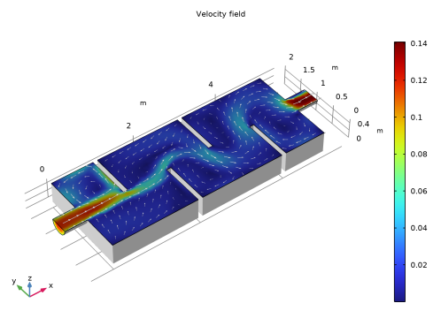
Results
Three plots are automatically created, one slice plot for the velocity, one pressure surface plot on the walls and one boundary plot of the wall lift-off in viscous units for the wall functions. The last one is important since it gives an indication of how well resolved the flow is at the walls. See Theory for the Turbulent Flow Interfaces in the CFD Module User’s Guide for further details on wall functions.
The following steps reproduce Figure 11.
First, create a dataset that corresponds to the nonwall boundaries.
Datasets
1
2
Velocity (spf)
1
2
3
4
5
6
7
-
-
8
9
10
-
-
-
11
12
13
-
-
14
Also reproduce Figure 12 as follows.
1
3D Plot Group 4
1
2
3
4
5
-
-
-
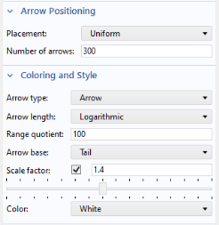
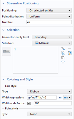
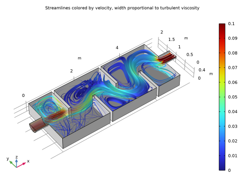
In the Width expression text field, type spf.nuT*1[s/m]. The width of the streamlines is set to the local value of the turbulent viscosity and the factor 1[s/m] is used to get the right dimension.
-
6
7
-
-
-
8
9
-
-
In the Title text area, type Streamlines colored by velocity. Width proportional to turbulent viscosity.
10
11
This concludes the introduction to the COMSOL CFD Module.