The Partial Fraction Fit function is used to fit frequency-dependent data for use in time domain simulations. Specific for acoustics applications, it can be frequency-dependent admittance data used with the Impedance condition in The Pressure Acoustics, Transient Interface or The Pressure Acoustics, Time Explicit Interface and frequency-dependent data for the equivalent density and compressibility used for the Poroacoustics model in the The Pressure Acoustics, Time Explicit Interface.

Let F(ω) be a complex-valued function of angular frequency ω = 2πf. An approximate analytical representation of its time-domain original, F(t), can be retrieved from a rational approximation of F(ω) that is defined on the whole complex plane:

Indeed, each fraction term on the right-hand side of Equation 2-8 corresponds to an exponential decay in the time domain

where L-1 is the inverse Laplace transform and H(t) is the Heaviside step function.

The causality and reality conditions are fulfilled if F∞ is real; the residues, Ak, and poles, αk, are either real or come in complex-conjugate pairs; and (for the exponentials in Equation 2-9 to decay as the time increases). That is

where NR and NC are the numbers of pure real poles and complex-conjugate pole pairs, respectively.

The partial fraction approximation (expansion) obtained through the built-in Partial Fraction Fit function approximates a given function of frequency within a given frequency range, for example, from fmin to fmax. The form given by Equation 2-10 ensures that the reality condition is fulfilled. This is not always the case for the causality and passivity conditions. However, the Partial Fraction Fit function has the necessary tools that can be used to make the result fulfill the causality and reality conditions, thus making the time-domain impedance boundary condition physical.

The Partial Fraction Fit function fits the input data based on a given tolerance (default 10−3), number of iterations (default 3), or either of those. The options are found in the Advanced section. A higher tolerance error results in a higher degree, N, of the polynomials in Equation 2-8 and therefore a larger number of terms in the expansion Equation 2-10. The default tolerance provides a balance between the approximation accuracy and the number of terms in the expansion, thus the computation costs when the expansion is used in an impedance boundary condition. On the other hand, increasing the tolerance may yield better results. The iteration-based approach can come in handy if you would like to see how the fit evolves as the number of iterations, and thus the degree of the polynomials, increases. This option is also useful when the fitted data is polluted by noise. 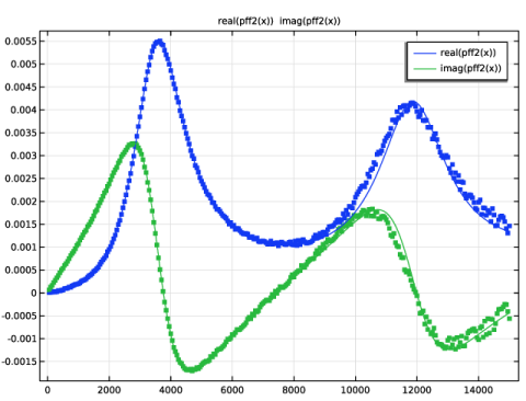Figure 2-12 and Figure 2-13 demonstrate the situation, where the functionality is used to fit the same “clean” and “noisy” admittance data, respectively.

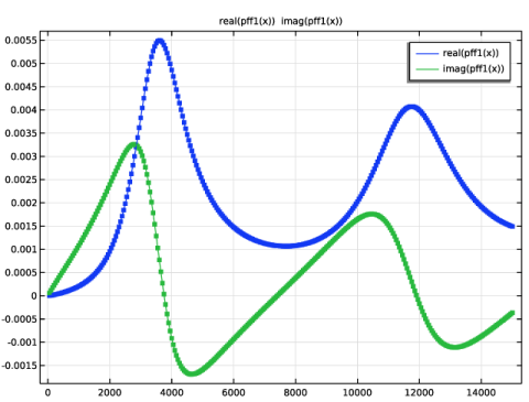
The “clean” data is fitted with the tolerance of 10−3 and results in 3 real poles and 3 pairs of complex-conjugate poles. The “noisy” data is fitted with 3 iterations, which results in a fairly good approximation with 1 real pole and 2 pairs of complex-conjugate poles. If the tolerance-based criterion is used instead, the approximant will interpolate the polluted data to reach the given tolerance. This will result in an undesired fit with an enormous number of poles. For example, fitting the “noisy” data with the tolerance of 10−2 yields 70 pairs of complex-conjugate poles, some of them located very close to the imaginary axis.

The violation of the causality condition takes place when one or more poles in the partial fraction expansion have positive real part (that is, they are unstable), which can usually happen to the pure real poles. Click the Flip Poles button to flip the unstable poles to the left half plane and circumvent the issue. The residues will be recomputed and updated automatically.

Sometimes the poles (stable or not) lie close to the zeros of the approximant. They can be judged by the residues that have absolute values much smaller than the others, which indicates that the poles and zero nearly cancel, and their influence is often localized. Such poles often referred to as spurious poles or Froissart doublets. You can either discard them (delete the row on the list) with the following update of the residues by clicking the Update Residues button; or run the algorithm with the option Automatically detect and remove Froissart doublets enabled. Note that results can be different. In contrast to simply discarding spurious poles, the detection procedure finds residues with absolute values lower than the given threshold compared to the residue with the maximum absolute value and performs a cleanup recomputing the approximant. If desired, change the threshold value in the Threshold field (default: 10−3).

Real-valued poles correspond to a pure exponential decay. It is common to get expansions with only real-valued poles when fitting the equivalent density and compressibility used in Poroacoustic as they describe the dissipative nature of porous media. For the admittance data used for the Impedance boundary condition, the typical behavior is locally-resonant and therefore complex-conjugate pole pairs are common.

It is important that the approximants fulfill all three conditions. However, sometimes there are poles (usually pure real) with the absolute value much larger than that of the others. This results in a stiff ODE, which affects the stability of the time-integration scheme. Specifically, the The Pressure Acoustics, Time Explicit Interface physics interface relies on explicit time-integration schemes. The time step is deduced solely from the minimum mesh element size in a model and the speed of sound. This time step can be too large to achieve a stable solution of the ODE. For the Impedance condition, used in the The Pressure Acoustics, Transient Interface, this is not an issue as it relies on an implicit time integration method that does not exhibit the same stability challenges.