The Port boundary condition is used to excite and absorb acoustic waves that enter or leave waveguide structures, like a duct or channel, in an acoustic model. A given port condition supports one specific propagating mode. To provide the full acoustic description, combine several port conditions on the same boundary. Make sure that all propagating modes in the studied frequency range are included (all modes that have a cutoff frequency in the frequency range). By doing this, the combined port conditions provide a superior nonreflecting or radiation condition for waveguides to, for example, the
Plane Wave Radiation condition or a perfectly matched layer (PML) configuration. The same port boundary condition feature should not be applied to several waveguide inlets/outlets. The port condition supports S-parameter (scattering parameter) calculation but it can also be used as a source to just excite a system. The
Port boundary condition exists for 3D, 2D, and 2D axisymmetric models.
|
|
|
•
|
Absorptive Muffler: Application Library path Acoustics_Module/Automotive/absorptive_muffler
|
|
where the summation “i” is over all ports on the given boundary “
bnd”,
Sij is the scattering parameter,
Ain is the amplitude of the incident field (at port “
j”),
φ is the phase of the incident field, and
pi is the mode shape of the
ith port. The mode shape
pi is normalized to have either a unit maximum amplitude or a unit power (see the normalization option in the
Global Port Settings section). This means that the scattering parameter
Sij defines the amplitude of mode
i when a system is exited at port
j (with mode
j). This corresponds to a multimode expansion of the solution on the given port. The scattering parameters are automatically calculated when an acoustic model is set up with just one port exciting the system. To get the full scattering matrix
The Port Sweep Functionality can be used.
|
|
An evaluation group for the Scattering Coefficient exists as a Predefined Plot. When evaluating, change the Data Series Operation for the port sweep parameter ( PortName) to Sum to get the proper data formatting.
|
Enter a unique Port name. Only nonnegative integer numbers can be used as
Port name as it is used to define the elements of the S-parameter matrix. The numeric port names are also required for port sweep functionality. The port name is automatically incremented by one every time a port condition is added.
Select a Type of port:
User defined (the default),
Numeric,
Circular,
Annular,
Rectangular,
Slit, or
User defined (nondispersive). Depending on the selection, different options appear in the
Port Mode Settings section (see below). Use the
Circular,
Annular, and
Rectangular for ports with the given cross section in 3D, the
Circular and
Annular options in 2D Axisymmetric, and the
Slit option in 2D. If the port has a different cross section, then either use the
User defined, the
Numeric, or the
User defined (nondispersive) port options. The
User defined or the
Numeric options can be used in cases where, for example, the waveguide is lined (an impedance is applied at the outer boundary).
|
•
|
For User defined enter user defined expressions for the Mode shape pn and the Mode wave number kn (SI unit: rad/m). The modes shape will automatically be scaled before it is used in the port condition. The normalized mode shape can be visualized by plotting acpr.port1.pn (here for Port 1, and so on). Use the user defined option to enter a known analytical expression or to use the solution from The Pressure Acoustics, Boundary Mode Interface. The solutions from the boundary mode analysis can be referenced using the withsol() operator.
|
|
|
The User defined option can be used to easily define a plane-wave mode. Simply enter 1 for the mode shape and acpr.k as the mode wave number.
|
|
•
|
The Numeric port option is used for waveguide cross sections that are neither circular nor rectangular. In this case, a boundary mode problem is solved on the port face to compute the desired propagating mode. This option requires the use of a Boundary Mode Analysis step in the study. It should be placed before the Frequency Domain step. In the study, add one Boundary Mode Analysis step for each Numeric port and make sure to reference the proper Port name in the study step.
|
Select the Mode wave number from option to decide how the mode wave number
kn is determined:
|
-
|
In general, for a model with losses, use the default Out-of-plane wave number option; then the wave number is taken from the Boundary Mode Analysis step. In this case, it is not possible to perform a frequency sweep in the Frequency Domain study step. Only one frequency can be used and it should correspond to the Mode analysis frequency entered in the Boundary Mode Analysis step(s). One option is to add a Parametric Sweep and define a parameter for the frequency used in both the steps. In this case, care should be taken when setting up the search criteria in the mode analysis.
|
|
-
|
For a model without any losses (nondispersive), select the Computed lossless mode cutoff frequency option. In this case, a frequency sweep is possible. The Boundary Mode Analysis should only be carried out at the highest frequency in the sweep. The wave number is computed analytically for all the other frequencies.
|
|
|
When the Numeric port option is used and the boundary mode analysis is run, the boundary conditions from the Pressure Acoustics model are automatically inherited in the boundary problem. For this automatic procedure, there is only support for the Sound Hard Boundary (Wall), Symmetry, Pressure, and Sound Soft conditions. If you need a more complex behavior, use the Pressure Acoustics, Boundary Mode interface in combination with the User defined port type.
|
|
•
|
The Circular port option is used for a port with a circular cross section. Enter the Mode number, azimuthal m (in 3D) and the Mode number, radial n to define the mode captured by the port. In 3D, also right-click the Port condition to add the Port Reference Axis when the Circular port type is selected. In 3D, also select the Azimuthal angle dependency as Sine (the default) or Cosine. This option is used to add the two orthogonal modes that exist for a given azimuthal mode number, add a new Port feature for each variant. The cutoff frequency of the mode can be evaluated in Results using the variable acpr.port1.fc (here for Port 1, and so on). 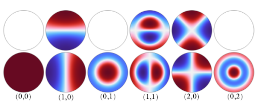
|
|
•
|
The Annular port option is used for a port with an annular cross section. Enter the Mode number, azimuthal m (in 3D) and the Mode number, radial n to define the mode captured by the port. In 3D, also right-click the Port condition to add the Port Reference Axis when the Annular port type is selected. In 3D, also select the Azimuthal angle dependency as Sine (the default) or Cosine. This option is used to add the two orthogonal modes that exist for a given azimuthal mode number; add a new Port feature for each variant. Also enter the Tolerance (default value 1e-8) used when computing the shape of the analytical modes (used for solving the associated Bessel-like equation). The default value is in general a good choice. The cutoff frequency of the mode can be evaluated in Results using the variable acpr.port1.fc (here for Port 1, and so on). 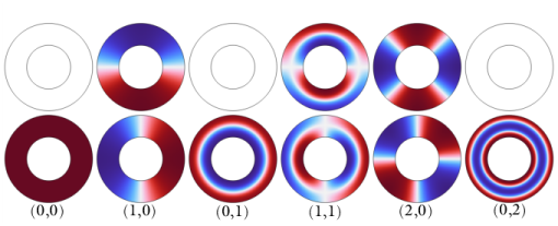
|
|
|
For the Annular option, if performing a parametric sweep over the port mode numbers m or n, only the Parametric Sweep can be used. The Auxiliary sweep option cannot be used, for this specific case.
|
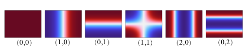
The Rectangular port option, only available in 3D, is used for a port with a rectangular cross section. Enter the
Mode number, longest side m and the
Mode number, shortest side n to define the mode captured by the port.
|
•
|
The Slit port option is only valid in 2D geometries. Enter the Mode number m to define the mode captured by the port.
|
|
•
|
The User defined (nondispersive) option is useful for models without losses (nondispersive waveguides). In this case, the mode shape remains constant over a frequency sweep and only the mode wave number kn changes. Enter an expression for the user-defined Mode shape pn; then enter the Mode wave number k0 and the Mode analysis frequency f0 at which the mode wave number k0 is defined. The wave number kn for a given frequency is then automatically computed and used for setting up the port.
|
Select the Port area as
Use symmetries (the default) or
Selected boundaries.
|
•
|
When Use symmetries is selected, symmetry conditions adjacent to the port will automatically be taken into account if the Port area multiplication factor is set to Automatic (the default); if set to User defined, enter the area multiplication factor Ascale manually.
|
|
•
|
When Selected boundaries is selected, the port will have the area of the selected boundaries, without taking any symmetry conditions into account.
|
|
|
The Port condition can only be applied to connected boundaries and the boundaries should typically be coplanar. The port condition can in principle be applied to a curved continuous boundary, but care should be taken that the setup is mathematically and physically consistent.
|
|
|
The Port boundary conditions should in general be placed at least one waveguide diameter from other geometry features to ensure that only a pure fully developed propagating wave exists at the port. Note also that the port condition does not treat possible evanescent waves.
|
Activate if the given port is excited by an incident wave of the given mode shape. For the first Port condition added in a model, the
Incident wave excitation at this port is set to
On. For subsequent conditions added, the excitation is set to
Off per default. If more than one port in a model is excited, the S-parameter calculation is not performed.
When the Incident wave excitation at this port is set to
On, then select how to define the incident wave. Set
Define incident wave to
Amplitude (the default) or
Power.
|
•
|
For Amplitude, enter the amplitude  (SI unit: Pa) of the incident wave. This is in general defined as the maximum amplitude for a given mode shape.
|
|
•
|
For Power, enter the power  (SI unit: W) of the incident wave. This is in general defined as the RMS power of the incident wave.
|
|
•
|
For both options, enter the phase φ (SI unit: rad) of the incident wave. This phase contribution is multiplied with the amplitude defined by the above options. The Amplitude input can be a complex number.
|
Note that when the Activate port sweep option is selected at the physics level, the options in the
Incident Mode Settings section are deactivated. This is because this option automatically sends in a mode of unit amplitude, sweeping through one port at a time.
|
|
For the Circular and Rectangular options make sure to only select modes that are actually symmetric according to the symmetry planes.
|
To display this section, click the Show More Options button (

) and select
Advanced Physics Options.
The port sweep functionality is used to reconstruct the full scattering matrix Sij by automatically sweeping the port excitation through all the ports included in the model. When the port sweep is activated, the options in the
Incident Mode Settings in the port conditions are deactivated and COMSOL controls which port that is excited with an incident mode.
The port sweep functionality is activated at the main physics interface level by selecting Activate port sweep in the
Global Port Settings section. Enter the
Sweep parameter name, the default is
PortName. Create a parameter with the same name under
Global Definitions >
Parameters 1. This is the name of the parameter to be used in a parametric sweep, here it should represent the
Port name integer values (defined when adding the port conditions). Add a parametric sweep study step and run the sweep over the
PortName parameter with an integer number of values representing all the ports in the model. Once the model is solved the full scattering matrix can be evaluated using the defined global variables
acpr.S11,
acpr.S21,
acpr.S12, and so on. The transmission loss (TL) between two given ports is also computed, for example, the variable for the TL loss from port 1 to 2 is given by
acpr.TL_12.
If only two ports are added to the pressure acoustics model, COMSOL also automatically computes the transfer matrix (two-port representation) of the system (variables acpr.T11,
acpr.T12,
acpr.T21,
acpr.T22) and the impedance matrix of the system (
acpr.Z11,
acpr.Z12,
acpr.Z21,
acpr.Z22). These expressions are only true if plane wave modes are used.
|
|
|
•
|
An evaluation group for the Scattering Coefficient exists as a Predefined Plot. The Global Matrix Evaluation is used to evaluate the full scattering matrix acpr.S. When evaluating, change the Data Series Operation for the port sweep parameter (typically PortName) to Sum to get the proper data formatting.
|
|
•
|
An Predefined Plot evaluation group also exists for the Transfer Matrix. This plot evaluates the real and imaginary parts of the four matrix components separately. The output format can readily be exported to a file and used as interpolation data for subsequent use in other models, for example, in connection to a Lumped Port condition.
|
|