J-integrals
The J-integral is a path independent integral that can be used to characterize the severity of the stress state at the crack tip, both for linear and some nonlinear materials. You can compute J-integrals by adding one or more J-integral subnodes under Crack.
Originally, the J-integral concept was derived for 2D, in which case it was sufficient to integrate certain functions of stress and strain along an arbitrary curve from one boundary of the crack to the other.
Figure 2-29: Example of a J-integral path.
There are some important assumptions when computing the J-integral:
In cases where the J-integral is not applicable, you can instead use the Virtual Crack Extension Method method.
You can specify the integration path as a circle with a given radius, in which case it cuts the mesh elements at arbitrary locations. In 2D, you can also select a sequence of internal or external boundaries describing the path. It is recommended that you evaluate more than one path to assess the accuracy of the solution.
The importance of this method is that stresses and strains far from the singular fields at the crack tip are used for the evaluation.
J-integrals can be computed also in 3D, but there are some complications. In the 3D case, the value of J will vary along the crack front. The local value is computed by a similar path integral, which then must be placed in the plane perpendicular to the crack front. This is automatically handled by the J-integral node. The J-integral in 3D should be considered as a continuous function along the crack front.
In 3D, there is also a surface integral contribution which needs to be computed for the area that is enclosed by the curve. Unfortunately, this causes the singular field to enter the integration, a fact that reduces accuracy. In addition, the computational effort increases significantly. Evaluations of J-integrals in 3D can take a noticeable time.
Another problem, that exists only in 3D, occurs if the crack front terminates at a free boundary. If the crack front is not perfectly perpendicular to the free boundary, the integration path will not entirely remain inside the solid domain. This is manifested as spurious results close to the free boundary.
Predefined Plots
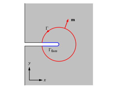
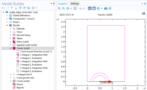
When J-integral nodes are present, they will generate predefined plots. These plots reside in a Cracks plot group. The contents of the plots differ significantly between 2D and 3D, as described below.
2D
The integration paths are plotted as magenta curves. An arrow shows the crack growth direction. At the crack tips, the value from the last J-integral node is printed. An example is shown in Figure 2-30.
Figure 2-30: Predefined plot for a 2D case with a crack in a symmetry plane. Three integration paths are shown; 2 circular and one along boundaries.
3D
In 3D, the integration paths are shown as transparent gray boundaries. The actual integration paths are located where this boundary is intersected by planes perpendicular to the crack front.
A colored arrow plot shows the crack growth direction, as well as the local value of the J-integral as computed in the last J-integral node. An example is shown in Figure 2-31.
Figure 2-31: Predefined plot for a case with a 3D crack in a symmetry plane. One integration path is used.
Default Evaluation Groups
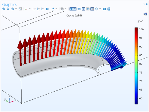
In both 3D and 2D, a predefined evaluation group, named Fracture Mechanics Results, is also generated. It contains a table with values of J-integrals and stress intensity factors for all integration paths. In 3D, however, only the maximum value of J along the crack front is reported.