The Semiconductor Interface includes quasi-Fermi level, density-gradient, logarithmic finite element formulations and a finite volume formulation. The formulation used is selected in the Discretization section since the shape functions that can be used are directly related to the formulation employed.

The finite volume formulation uses constant shape functions, whilst the logarithmic finite element formulations can use either linear or quadratic shape functions. In the different formulations the carrier concentration dependent variables (by default Ne and Ph) represent different quantities. In the finite volume formulations Ne = N and Ph = P, where N is the electron concentration and P is the hole concentration. For the logarithmic finite element formulation Ne = ln(N) and Ph = ln(P). For the quasi-Fermi level and density-gradient formulation, the quasi-Fermi levels for the electrons and holes are the dependent variables (by default Efn_ and Efp_).

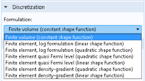
To change the formulation, first expand the Discretization section. Then under Discretization select a Formulation (as in Figure 2-1). Each formulation has advantages and disadvantages.

The finite volume discretization inherently conserves current. Consequently, it usually provides the most accurate result for the current density of the charge carriers. In order to enhance numerical stability, a Scharfetter–Gummel upwinding scheme is used for the charge carrier equations. Poisson’s equation is discretized using a centered difference scheme. When doing multiphysics simulations it is important to realize that the shape functions are constant. Consequently, fluxes cannot be evaluated using spatial derivatives of the dependent variables (for example, expressions such as d(V,x) evaluate to zero as V is represented by a constant shape function within each element). Flux quantities such as fields and currents can be evaluated and used in equations (both within the Semiconductor interface and in other physics interfaces) if the predefined variables from Table 2-1 are used in expressions:

Any variables that involve expressions directly derived from the variables in Table 2-1 can also be used in expressions, for example, the electric field, semi.normE, semi.EX, semi.EY, semi.EZ, or the total current, semi.normJ, semi.JX, semi.JY, semi.JZ.

The logarithmic finite element formulation typically solves faster than the finite volume formulation. One reason is that, for an identical mesh, the finite element method with linear shape functions typically results in fewer degrees of freedom. In 2D, for triangular mesh elements, the number of degrees of freedom for the finite element method with linear shape functions is approximately half that for a finite volume discretization. Coupling to other physics interfaces is straightforward and variables can be differentiated using the d operator.