You are viewing the documentation for an older COMSOL version. The latest version is
available here.
Use the Release node to release rays within domains based on arbitrary expressions or based on the positions of the mesh elements.
This section is only available when the Allow multiple release times check box has been selected in the physics interface
Advanced Settings section. Enter
Release times (SI unit: s) or click the
Range button (

) to select and define a range of specific times. At each release time, rays are released with initial position and ray direction vector as defined next.
Select an Initial position:
Density (the default) or
Mesh based.
For Density enter a value for the
Number of rays per release N (dimensionless). The default is
100. Then enter a value or expression for the
Density proportional to ρ (dimensionless). The default is
1.
The Density proportional to ρ can be an expression rather than a number; the resulting ray distribution approximately has a number density that is proportional to this expression. The resulting distribution looks a bit random, and it depends on the order in which the mesh elements are numbered. The distribution is probably not exactly the same in different COMSOL Multiphysics versions, but the total number of rays released is always
N.
|
|
The Density proportional to expression must be strictly positive.
|
Select a Release distribution accuracy order between
1 and
5 (the default is
5), which determines the integration order that is used when computing the number of rays to release within each mesh element. The higher the accuracy order, the more accurately rays will be distributed among the mesh elements.
The Position refinement factor (default
0) must be a nonnegative integer. When the refinement factor is
0, each ray is always assigned a unique position, but the density is taken as a uniform value over each mesh element. If the refinement factor is a positive integer, the distribution of rays within each mesh element is weighted according to the density, but it is possible for some rays to occupy the same initial position. Further increasing the
Position refinement factor increases the number of evaluation points within each mesh element to reduce the probability of multiple rays occupying the same initial position.
For Mesh based the rays are released from a set of positions determined by a selection of geometric entities (of arbitrary dimension) in the mesh. Given a
Refinement factor between 1 and 5, the centers of the refined mesh elements are used. Thus, the number of positions per mesh element is
refine^dim, except for pyramids, where it is
(4*refine2-1)*refine/3.
Select an option from the Ray direction vector list:
Expression (the default),
Spherical,
Hemispherical,
Conical, or
Lambertian (3D only).
|
•
|
For Expression a single ray is released in the specified direction. Enter coordinates for the Ray direction vector L0 (dimensionless) based on space dimension.
|
|
•
|
For Spherical a number of rays are released at each point, sampled from a spherical distribution in wave vector space. Enter the Number of rays in wave vector space Nw (dimensionless). The default is 50.
|
|
•
|
For Hemispherical a number of rays are released at each point, sampled from a hemispherical distribution in wave vector space. Enter the Number of rays in wave vector space Nw (dimensionless). The default is 50. Then enter coordinates for the Hemisphere axis r based on space dimension.
|
|
•
|
For Conical a number of rays are released at each point, sampled from a conical distribution in wave vector space. Enter the Number of rays in wave vector space Nw (dimensionless). The default is 50. Then enter coordinates for the Cone axis r based on space dimension. Then enter the Cone angle a (SI unit: rad). The default value is π/3 radians.
|
|
•
|
The Lambertian option is only available in 3D. A number of rays are released at each point, sampled from a hemisphere in wave vector space with probability density based on the cosine law. Enter the Number of rays in wave vector space Nw (dimensionless). The default is 50. Then enter coordinates for the Hemisphere axis r based on space dimension.
|
If Conical is selected in a 3D model, select an option from the
Conical distribution list:
|
•
|
Uniform density (the default): rays are released with polar angles from 0 to the specified cone angle. The rays are distributed in wave vector space so that each ray subtends approximately the same solid angle.
|
|
•
|
Specify polar and azimuthal distributions: specify the Number of polar angles Nθ (dimensionless) and the Number of azimuthal angles Nφ (dimensionless). Rays are released at uniformly distributed polar angles from 0 to the specified cone angle. A single axial ray ( θ = 0) is also released. For each value of the polar angle, rays are released at uniformly distributed azimuthal angles from 0 to 2π. Unlike other options for specifying the conical distribution, it is not necessary to directly specify the Number of rays in wave vector space Nw (dimensionless), which is instead derived from the relation Nw = Nθ × Nφ + 1.
|
|
•
|
Hexapolar: specify the Number of polar angles Nθ (dimensionless). In this distribution, for each release point, one ray will be released along the cone axis. Six rays are released at an angle α/Nθ from the cone axis, then 12 additional rays at an angle of 2 α/Nθ, and so on. The total number of ray directions in the distribution is Nw = 3 Nθ( Nθ + 1) + 1.
|
|
•
|
Flat: rays are released in a flat fan shape within the specified angle.
|
|
•
|
Marginal rays only: the rays are all released at an angle α with respect to the cone axis. The rays are released at uniformly distributed azimuthal angles from 0 to 2π.
|
|
•
|
Marginal and axial rays only: the rays are all released at an angle α with respect to the cone axis, except for one ray which is released along the cone axis. The marginal rays are released at uniformly distributed azimuthal angles from 0 to 2π.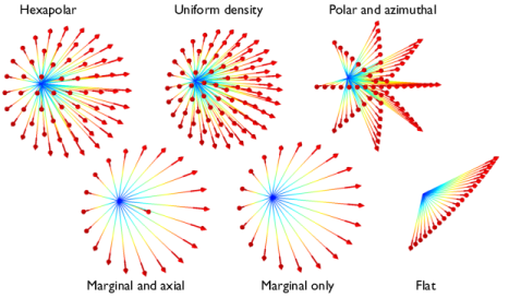
|
In 3D for the Conical distribution you can also let the
Transverse direction be
Automatic (the default) or
User defined. For
User defined enter the components of
et. This controls, for example, the orientation of the ray fan when
Flat is selected.
For Spherical,
Hemispherical,
Conical, and
Lambertian, select an option from the
Sampling from Distribution list:
Deterministic (the default) or
Random. If
Deterministic is selected, the initial ray direction vectors are computed using an algorithm that seeks to distribute the rays as evenly as possible in wave vector space. This algorithm will give the same initial ray directions whenever the study is run. If
Random is selected, the initial direction of each ray is sampled from a probability distribution in wave vector space using pseudorandom numbers. The result may be the same when rerunning the study multiple times on the same computer, but the solution is likely to be different on different architectures.
This section is available when Polychromatic, specify frequency is selected from the
Wavelength distribution of released rays list in the physics interface
Ray Release and Propagation section.
Select a Distribution function:
None (the default),
Normal,
Lognormal,
Uniform,
Blackbody, or
List of values.
When None is selected, enter an initial value
ν0 (SI unit: Hz). The default value is
4.54 × 10¹⁴ Hz.
Select Normal to create a normal distribution function,
Lognormal to create a log-normal distribution function,
Uniform to create a uniform distribution function, or
Blackbody to sample values according to Planck’s law for blackbody radiation. For any of these distributions, select an option from the
Sampling from distribution check box:
Deterministic (the default) or
Random. For
Random sampling the mean and standard deviation may not be exactly equal to the expected values but will statistically converge as the number of rays is increased. The
Number of values sets the number of values that are sampled from the distribution function at each release point.
For the Normal or
Lognormal distribution enter a user-defined
Mean ray frequency (default
4.54 × 10¹⁴ Hz) and
Ray frequency standard deviation (default
1014 Hz). For the
Uniform distribution enter the
Minimum ray frequency νmin (default
4.3 × 10¹⁴ Hz) and
Maximum ray frequency νmax (default
7.5 × 10¹⁴ Hz). Select
List of values to enter a list of distinct frequency values.
For Blackbody, enter the
Blackbody temperature Tbb (SI unit: K). The default value of 5780 K is an approximate value for treating the sun as a blackbody radiation source. Then select an option from the
Distribution type list:
Specify fraction of total emissive power (the default), or
Specify bandwidth.
|
•
|
If Specify fraction of total emissive power is selected, enter the Fraction of total emissive power fbb (dimensionless). The default is 0.95.
|
|
•
|
If Specify bandwidth is selected, enter the Minimum ray frequency νmin and Maximum ray frequency νmax (SI unit: Hz). The defaults are 4.3 × 10¹⁴ Hz and 7.5 × 10¹⁴ Hz, respectively.
|
This section is available when Polychromatic, specify vacuum wavelength is selected from the
Wavelength distribution of released rays list in the physics interface
Ray Release and Propagation section.
Select a Distribution function:
None (the default),
Normal,
Lognormal,
Blackbody,
Uniform, or
List of values.
When None is selected, enter a value or expression for the
Vacuum wavelength λ0 (SI unit: m). The default is
660 nm. All rays released by this feature will have the same wavelength.
Select Normal to create a normal distribution function,
Lognormal to create a log-normal distribution function,
Uniform to create a uniform distribution function, or
Blackbody to sample values according to Planck’s law for blackbody radiation. For any of these distributions, select an option from the
Sampling from distribution check box:
Deterministic (the default) or
Random. For
Random sampling the mean and standard deviation may not be exactly equal to the expected values but will statistically converge as the number of rays is increased. The
Number of values sets the number of values that are sampled from the distribution function at each release point.
For the Normal or
Lognormal distribution enter a user-defined
Mean vacuum wavelength (default
660 nm) and
Vacuum wavelength standard deviation (default
100 nm). For the
Uniform distribution enter the
Minimum vacuum wavelength λ0,min (default
400 nm) and
Maximum vacuum wavelength λ0,max (default
700 nm). Select
List of values to enter a list of distinct wavelength values directly.
For Blackbody, enter the
Blackbody temperature Tbb (SI unit: K). The default value of 5780 K is an approximate value for treating the sun as a blackbody radiation source. Then select an option from the
Distribution type list:
Specify fraction of total emissive power (the default), or
Specify bandwidth.
|
•
|
If Specify fraction of total emissive power is selected, enter the Fraction of total emissive power fbb (dimensionless). The default is 0.95.
|
|
•
|
If Specify bandwidth is selected, enter the Minimum vacuum wavelength λ0,min and Maximum vacuum wavelength λ0,max (SI unit: m). The defaults are 400 nm and 700 nm, respectively.
|
This section is available when the Compute phase check box is selected under the physics interface
Intensity Computation section. Enter an
Initial phase Ψ0 (SI unit: rad). The default value is
0.
This section is available when the ray intensity is solved for in the model and Expression is selected as the
Ray direction vector. Enter a value for the
Initial intensity I0 (SI unit: W/m
2). The default is
1000 W/m
2.
This section is available when the ray intensity is solved for in the model and Expression is selected as the
Ray direction vector. Select a
Wavefront shape. In 3D the available options are
Plane wave (the default),
Spherical wave, and
Ellipsoid. In 2D the available options are
Plane wave (the default) and
Cylindrical wave.
|
•
|
For a Spherical wave or Cylindrical wave, enter the Initial radius of curvature r0 (SI unit: m).
|
|
•
|
For an Ellipsoid, enter the Initial radius of curvature, 1 r1,0 (SI unit: m) and the Initial radius of curvature, 2 r2,0 (SI unit: m). Also enter the Initial principal curvature direction, 1 e1,0 (dimensionless).
|
|
|
For spherical and cylindrical waves the Initial radius of curvature must be nonzero. To release a ray such that the initial wavefront radius of curvature is zero, instead select a different option such as Conical from the Ray direction vector list.
|
Select an Initial polarization type:
Unpolarized (the default),
Fully polarized, or
Partially polarized.
Select an Initial polarization:
Along principal curvature direction (the default) or
User defined.
|
•
|
For Fully polarized and Partially polarized rays in 3D enter an Initial polarization parallel to reference direction a1,0 (dimensionless), Initial polarization perpendicular to reference direction a2,0 (dimensionless), and Initial phase difference δ0 (SI unit: rad).
|
|
•
|
For Fully polarized and Partially polarized rays in 2D enter an Initial polarization, in plane axy,1 (dimensionless), Initial polarization, out of plane az,0 (dimensionless), and Initial phase difference δ0 (SI unit: rad).
|
|
•
|
For User defined also enter an Initial polarization reference direction u (dimensionless).
|
For Partially polarized, also enter an
Initial degree of polarization P0 (dimensionless).
|
•
|
when Spherical, Hemispherical, or Conical is selected as the Ray direction vector.
|
Select an option from the Intensity initialization list:
Uniform distribution (the default) or
Weighted distribution. If any
Photometric Data Import nodes have been added to the model then they can also be selected from the list.
If Uniform distribution or
Weighted distribution is selected, enter a
Total source power Psrc (SI unit: W). The default is
1 W. In 2D, instead enter the
Total source power per unit thickness Psrc (SI unit: W/m). The default is
1 W/m. For
Weighted distribution, also enter an expression for the
Power weighting factor Pwt. The weighting factor may have any unit; the default expression is 1. The released rays will have initial intensity and power proportional to the weighting factor, while still adding up to the specified source power.
|
|
For example, if you release 1000 rays in a Spherical distribution with an initial power of 10 W, and enter a weighting factor of gop.niz+1, then the sum of the power over all released rays, gop.sum(gop.Q), will equal 10 W. Since gop.niz is the z-component of the ray direction vector, rays close to the z-axis will each have power of about 0.02 W, those around the negative z direction will have almost no power, and those in the xy-plane will each have power of about 0.01 W.
|
If any Photometric Data Import feature is selected from the list, the source power is instead obtained directly from the imported photometric data (IES) file. Enter values or expressions for the components of the
Photometric horizontal ph (dimensionless) and
Photometric zero pz (dimensionless). By default, these vectors point in the directions of the positive
x- and
z-axes, respectively.
|
|
The Photometric Data Import feature does not support the options TILT=INCLUDE or TILT=<FILENAME> that are included in some IES files. Only TILT=NONE is allowed.
|
For each of the Auxiliary Dependent Variable nodes added to the model, select a
Distribution function for the initial value of the auxiliary dependent variables and whether the initial value of the auxiliary dependent variables should be a scalar value or sampled from a distribution function.
When None is selected, enter an initial value. The symbol for the initial value is the auxiliary variable name followed by a subscript
0, so for the default name
rp the initial value has symbol
rp0.
For the initial value of the auxiliary dependent variables, select Normal to create a normal distribution function,
Lognormal to create a log-normal distribution function, or
Uniform to create a uniform distribution function. For any of these distributions, select an option from the
Sampling from distribution check box:
Deterministic (the default) or
Random. For
Random sampling the mean and standard deviation may not be exactly equal to the specified values but will statistically converge as the number of rays is increased. The
Number of values sets the number of values that are sampled from the distribution function at each release point.
For the Normal or
Lognormal distribution enter the
Mean (default
0) and
Standard deviation (default
1). For the
Uniform distribution enter the
Minimum (default 0) and
Maximum (default 1). Select
List of values to enter a set of numerical values directly.
By default auxiliary dependent variables are initialized after all other degrees of freedom. Select the Initialize before wave vector check box to compute the initial value of the auxiliary dependent variable immediately after computing the initial wave vectors of the rays. By selecting this check box it is possible to define the initial ray direction as a function of the auxiliary dependent variables.