Inlet
Use the Inlet node to release particles into the modeling domain from selected boundaries. The Nonlocal Accumulator subnode is available from the context menu (right-click the parent node) or from the Physics toolbar, Attributes menu.
Go to Release for information about the following sections: Release Times, Release Current Magnitude, Mass Flow Rate, Released Particle Properties, Initial Particle Temperature, Initial Particle Mass, Initial Multiplication Factor, Initial Value of Auxiliary Dependent Variables, and Advanced Settings.
Coordinate System Selection
It is possible to specify the initial particle velocity in terms of the global coordinates or in another coordinate system defined for the model Component. Select an option from the Coordinate system list. By default Global coordinate system is selected. If other coordinate systems are defined, they can also be selected from the list. When specifying the initial particle velocity (see the Initial Velocity section), velocity or direction components can be specified using the basis vectors of whichever coordinate system has been selected from the list.
When a coordinate system other than Global coordinate system is selected from the Coordinate system list, arrows will appear in the Graphics window to indicate the orientation of the basis vectors of the coordinate system on the selected boundaries.
Initial Position
Select an Initial position: Mesh based (the default), Uniform distribution (2D components) Projected plane grid (3D components), Density, or Random. Mesh Based, Density, and Random have the same settings as described for the Release node.
For 2D components, if Uniform distribution is selected, enter the Number of particles per release N (dimensionless). The default is 1. The union of the selected edges is divided into N segments of approximately equal length, and a particle is placed in the middle of each segment.
For 3D components, if Projected plane grid is selected, enter the Number of particles per release N (dimensionless). The default is 1. The particles are distributed on a plane grid in planes that are approximately tangential to the selected boundaries.
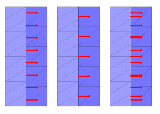
For inlets defined on identity pairs in an assembly, select an option from the Release particles from boundaries list: Source (the default), Destination, or Source and Destination. This option determines which boundary mesh to use when determining the initial particle positions. The mesh on either side of an inlet pair can be quite different, as shown in Figure 3-2.
Figure 3-2: Mesh-based release of particles from a source boundary (left), destination boundary (middle), or both source and destination (right). In each rectangle, the source boundary is on the side of the lighter-colored mesh.
Initial Velocity
Select an Initial velocity: Expression (the default), Kinetic energy and direction, Constant speed, hemispherical, Constant speed, cone, Constant speed, Lambertian (3D only), or Thermal.
For Expression enter expressions for the Initial particle velocity v0 (SI unit: m/s) based on space dimension. Select the Specify tangential and normal vector components check box to enter expressions for the initial velocity in terms of the tangential and normal directions at the surface.
When using The Particle Tracing for Fluid Flow Interface, enter a value or expression for the Velocity field u. If another physics interface that computes the velocity field is present, then this interface can be selected from the list.
For Kinetic energy and direction enter the Initial kinetic energy E0 (SI unit: J). The default is 1 keV. Then enter coordinates for the Initial particle direction L0 (dimensionless) based on space dimension. It is not necessary to normalize the components of the initial direction vector because this is done automatically when computing the initial velocity. Select the Specify tangential and normal vector components check box to enter expressions for the initial direction in terms of the tangential and normal directions at the surface.
The option Kinetic energy and direction is not supported for The Particle Tracing for Fluid Flow Interface.
For Constant speed, hemispherical enter a Speed v0 (SI unit: m/s), the Number of particles in velocity space Nvel (dimensionless), and the Hemisphere axis r. Select the Specify tangential and normal vector components check box to enter expressions for the hemisphere axis in terms of the tangential and normal directions at the surface.
For Constant speed, cone enter a Speed v0 (SI unit: m/s), the Number of particles in velocity space Nvel (dimensionless), the Cone axis r, and the Cone angle α (SI unit: rad). Select the Specify tangential and normal vector components check box to enter expressions for the cone axis in terms of the tangential and normal directions at the surface.
The Constant speed, Lambertian option is only available in 3D. Enter a Speed v0 (SI unit: m/s), the Number of particles in velocity space Nvel (dimensionless), and the Hemisphere axis r. The velocity distribution is a hemisphere in which the distribution of polar angles follows the cosine law, similar to the Diffuse scattering option for the Wall feature. Select the Specify tangential and normal vector components check box to enter expressions for the hemisphere axis in terms of the tangential and normal directions at the surface.
For Thermal, enter a value or expression for the Temperature T of the boundary (SI unit: K). The default is 293.15 K. If the temperature is computed by another physics interface in the model then it can be selected from the list. The Thermal option samples the initial particle velocity from a distribution in the same manner as the Thermal Reemission boundary condition. For more details see About the Boundary Conditions for the Particle Tracing Interfaces in the Theory for the Mathematical Particle Tracing Interface section.
 
When the Specify tangential and normal velocity components or Specify tangential and normal vector components check box is selected, arrows indicating the normal direction on the selected boundaries will appear in the Graphics window.
Note that the normal direction may be opposite the built-in variable for the boundary normal (for example, nx, ny, and nz) to ensure that a positive value causes particles to be released into the simulation domain. This often occurs when the Inlet is applied to exterior boundaries.
When the normal direction used by the Inlet feature is opposite the normal vector defined by the geometry, the tangential directions are similarly inverted to ensure that the boundary coordinate system is right-handed.
For Constant speed, hemispherical, Constant speed, cone, and Constant speed, Lambertian, select an option from the Sampling from distribution list: Deterministic (the default) or Random. If Deterministic is selected, the initial velocity is computed by sampling from the velocity distribution in a deterministic and reproducible manner. If Random is selected, the particle velocity is sampled from the distribution using pseudorandom numbers and may not always generate the same results.
For Constant speed, spherical, Constant speed, hemispherical, Constant speed, cone, and Constant speed, Lambertian, select the Allow nonuniform speeds in distribution check box to allow particles from the same release point to have different initial speeds. This check box has no effect on the initial velocity directions of the released particles, only their velocity magnitudes. If this check box is selected, expressions for the initial speed in terms of the particle index can return a unique value for each particle in the distribution.
For example, if Constant speed, hemispherical is selected from the Initial velocity list, the Allow nonuniform speeds in distribution check box is selected, and the expression for the initial speed is 2[m/s]*(random(pt.pidx)+0.5), then particles will be released with directions sampled from an isotropic hemisphere and with speeds sampled pseudorandomly between 0 and 2 m/s.