PDF

Turbulent Flow Through a Shell-and-Tube Heat Exchanger Cross Section
Introduction
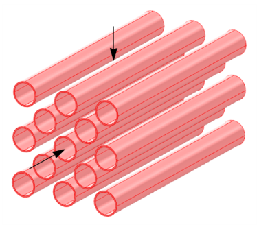
This example describes a part of a shell-and-tube heat exchanger (see Figure 1), where hot water enters from above. The cooling medium, commonly water, flows through the pipes and enters from the side. The tubes are assumed to be made of stainless steel.
Figure 1: A tube bundle from a shell-and-tube heat exchanger. The arrows indicate the flow directions.
Assuming that the cooling water is in abundant supply, the flow through the pipes has a constant temperature. Under that assumption, you can model this heat exchanger by a 2D model as shown in Figure 2, and the corresponding 2D domain appears in Figure 3. Note that the pipe interiors are not part of the domain because the model assumes the temperature to be constant there.
Figure 2: The dashed line marks the model region, which is shown in Figure 3.
Figure 3: The modeled 2D region.
The Need for a Turbulence Model
An important characteristic of the flow is the Reynolds number, Re, defined as
where U is a velocity scale, L is a length scale, and η is a kinematic viscosity. If the Reynolds number is low, no turbulence model is needed. If, on the other hand, the Reynolds number is high, then the flow is dominated by convection, and a turbulence model is necessary.
In this case, a suitable velocity scale is the mean inlet velocity, which is 1.5 m/s, and L is set to the pipe radius. Then, using standard values for water for the density and viscosity, the equation gives an approximate Reynolds number of 75,000, which is high enough to warrant the use of a turbulence model (see Ref. 1 for more information on flow regimes for different Reynolds numbers).
The following example demonstrates how to model a coupled fluid-thermal interaction problem with COMSOL Multiphysics, using the Nonisothermal Flow multiphysics coupling.
Model Definition
Solid and Fluid Heat Transfer — Including the Fluid Dynamics
The governing equations in this model are (Ref. 2Ref. 4)
The Nonisothermal Flow multiphysics coupling sets up both sets of equations together with the applicable couplings, making it easy to model the fluid-thermal interaction.
The model uses temperature-dependent properties for water and steel from the built-in material library. It incorporates the influence of the turbulent fluctuations on the temperature field by using the Kays–Crawford model for the turbulent Prandtl number (for details, see the section Turbulent Nonisothermal Flow Theory in the Heat Transfer Module User’s Guide). Furthermore, to account for the effect of mixing due to eddies, it is necessary to correct the fluid’s thermal conductivity. The turbulence results in an effective thermal conductivity, keff, according to the equation
where k is the fluid’s physical thermal conductivity and κT is the turbulent thermal conductivity. Furthermore, μT denotes the turbulent dynamic viscosity, Cp is the heat capacity, and PrT refers to the turbulent Prandtl number. Be careful not to confuse k in the meaning of thermal conductivity with k in the meaning of turbulent kinetic energy.
The boundary conditions for the problem are:
k-ε equations in the fluid domain:
-
-
-
-
-
-
-
-
-
Results for the Flow/Heat Model
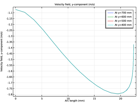
Figure 4 shows the velocity in the inlet of several segments in the middle of the computational domain. The flow field is periodic in the direction with the constant pressure drop of about 1350 Pa. (Figure 5).
Figure 4: Velocity at y = 400, 500, 600, and 700 mm.
Figure 5: Pressure at y = 400, 500, 600, and 700 mm.
Figure 6 depicts the temperature distribution and velocity streamlines in the segment. The heat transfer is strongly influenced by the details of the velocity field. Observe the low-temperature zones behind the pipes created by the recirculation zones.
Figure 7 shows the temperature profiles at y = 400, 500, 600, and 700 mm.
Figure 6: Temperature distribution in the segment.
Figure 7: Temperature distribution at y = 400, 500, 600, and 700 mm.
Notes About the COMSOL Implementation
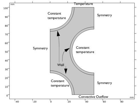
You start by performing an initial calculation for the single segment of the computational domain (Figure 8). Proceed by creating a linear array of the segments. The appropriate physical interface settings are automatically extended to all elements of the array.
Figure 8: Modeled segment of the heat exchanger with boundary conditions.
References
1. J.R. Welty, C.E. Wicks, and R.E. Wilson, Fundamentals of Momentum, Heat and Mass Transfer, 3rd ed, John Wiley & Sons, 1984.
2. B.E. Launder and D.B. Spalding, “The Numerical Computation of Turbulent Flows,” Computer Methods in Applied Mechanics, vol. 3, pp. 269–289, 1974.
3. D.C. Wilcox, Turbulence Modeling for CFD, 2nd ed, DCW Industries, 2000.
4. H.K. Versteeg and W. Malalasekera, An Introduction to Computational Fluid Dynamics, Prentice Hall, 1995.
Application Library path: Heat_Transfer_Module/Heat_Exchangers/turbulent_heat_exchanger
Modeling Instructions
From the File menu, choose New.
New
In the New window, click  Model Wizard.
Model Wizard
1
In the Model Wizard window, click  2D.
2
In the Select Physics tree, select Fluid Flow>Nonisothermal Flow>Turbulent Flow>Turbulent Flow, k-ε.
3
Click Add.
4
Click  Study.
In this model, the flow will be considered nearly incompressible and independent of temperature variations. Under these assumptions, the Stationary, One-Way NITF study performs best.
5
In the Select Study tree, select Preset Studies for Selected Multiphysics>Stationary, One-Way NITF.
6
Global Definitions
Parameters 1
1
In the Model Builder window, under Global Definitions click Parameters 1.
2
In the Settings window for Parameters, locate the Parameters section.
3
Geometry 1
1
In the Model Builder window, under Component 1 (comp1) click Geometry 1.
2
In the Settings window for Geometry, locate the Units section.
3
From the Length unit list, choose mm.
Now draw the segment of the heat exchanger that forms the model geometry for the first simulation.
Rectangle 1 (r1)
1
In the Geometry toolbar, click  Rectangle.
2
In the Settings window for Rectangle, locate the Size and Shape section.
3
In the Width text field, type 50.
4
In the Height text field, type 100.
5
Click  Build Selected.
Circle 1 (c1)
1
In the Geometry toolbar, click  Circle.
2
In the Settings window for Circle, locate the Size and Shape section.
3
In the Radius text field, type 27.5.
4
Click  Build Selected.
Circle 2 (c2)
1
In the Geometry toolbar, click  Circle.
2
In the Settings window for Circle, locate the Size and Shape section.
3
In the Radius text field, type 25.
4
Click  Build Selected.
Difference 1 (dif1)
1
In the Geometry toolbar, click  Booleans and Partitions and choose Difference.
2
3
In the Settings window for Difference, locate the Difference section.
4
Click to select the  Activate Selection toggle button for Objects to subtract.
5
6
Click  Build Selected.
Copy 1 (copy1)
1
In the Geometry toolbar, click  Transforms and choose Copy.
2
3
In the Settings window for Copy, locate the Displacement section.
4
In the x text field, type 0 50.
5
In the y text field, type 100 50.
6
Click  Build Selected.
Union 1 (uni1)
1
In the Geometry toolbar, click  Booleans and Partitions and choose Union.
2
Click in the Graphics window and then press Ctrl+A to select all objects.
3
In the Settings window for Union, click  Build Selected.
Delete Entities 1 (del1)
1
In the Model Builder window, right-click Geometry 1 and choose Delete Entities.
2
In the Settings window for Delete Entities, locate the Entities or Objects to Delete section.
3
From the Geometric entity level list, choose Domain.
4
On the object uni1, select Domains 1, 2, 5, 7, 8, and 10 only.
It might be easier to select the domains by using the Selection List window. To open this window, in the Home toolbar click Windows and choose Selection List. (If you are running the cross-platform desktop, you find Windows in the main menu.)
5
In the Geometry toolbar, click  Build All.
You should now see the following geometry.
Add Material
1
In the Home toolbar, click  Add Material to open the Add Material window.
2
Go to the Add Material window.
3
In the tree, select Built-in>Steel AISI 4340.
4
Click Add to Component in the window toolbar.
5
In the tree, select Built-in>Water, liquid.
6
Click Add to Component in the window toolbar.
7
In the Home toolbar, click  Add Material to close the Add Material window.
Materials
Steel AISI 4340 (mat1)
1
In the Model Builder window, under Component 1 (comp1)>Materials click Steel AISI 4340 (mat1).
2
Water, liquid (mat2)
1
In the Model Builder window, click Water, liquid (mat2).
2
3
In the Settings window for Material, locate the Geometric Entity Selection section.
4
Click  Create Selection.
5
In the Create Selection dialog box, type Water in the Selection name text field.
6
Heat Transfer in Fluids (ht)
Set the reference temperature to an estimated value of T_in where the flow operates.
1
In the Model Builder window, under Component 1 (comp1) click Heat Transfer in Fluids (ht).
2
In the Settings window for Heat Transfer in Fluids, locate the Physical Model section.
3
In the Tref text field, type T_in.
Solid 1
1
In the Physics toolbar, click  Domains and choose Solid.
2
Turbulent Flow, k-ε (spf)
The density variations are small enough to consider the fluid as incompressible. Change the compressibility option accordingly in the physics interface. The reference temperature is set in the Heat Transfer interface.
1
In the Model Builder window, under Component 1 (comp1) click Turbulent Flow, k-ε (spf).
2
In the Settings window for Turbulent Flow, k-ε, locate the Physical Model section.
3
From the Compressibility list, choose Incompressible flow.
4
Locate the Domain Selection section. From the Selection list, choose Water.
Inlet 1
1
In the Physics toolbar, click  Boundaries and choose Inlet.
2
3
In the Settings window for Inlet, locate the Velocity section.
4
Click the Velocity field button.
5
Specify the u0 vector as
Symmetry 1
1
In the Physics toolbar, click  Boundaries and choose Symmetry.
2
Outlet 1
1
In the Physics toolbar, click  Boundaries and choose Outlet.
2
Heat Transfer in Fluids (ht)
In the Model Builder window, under Component 1 (comp1) click Heat Transfer in Fluids (ht).
Inflow 1
1
In the Physics toolbar, click  Boundaries and choose Inflow.
2
3
In the Settings window for Inflow, locate the Upstream Properties section.
4
In the Tustr text field, type T_in.
Outflow 1
1
In the Physics toolbar, click  Boundaries and choose Outflow.
2
Temperature 1
1
In the Physics toolbar, click  Boundaries and choose Temperature.
2
3
In the Settings window for Temperature, locate the Temperature section.
4
In the T0 text field, type T_pipe.
Mesh 1
1
In the Model Builder window, under Component 1 (comp1) click Mesh 1.
2
In the Settings window for Mesh, locate the Physics-Controlled Mesh section.
3
From the Element size list, choose Fine.
4
Right-click Component 1 (comp1)>Mesh 1 and choose Edit Physics-Induced Sequence.
Size 2
1
In the Model Builder window, under Component 1 (comp1)>Mesh 1 click Size 2.
2
In the Settings window for Size, locate the Element Size section.
3
Click the Custom button.
4
Locate the Element Size Parameters section.
5
Select the Maximum element size check box. In the associated text field, type 0.5.
6
Click  Build All.
Study 1
Solve the problem for a single heat exchanger segment.
1
In the Home toolbar, click  Compute.
Results
Velocity (spf)
The default plots show the velocity, the wall resolution, and the temperature distribution in the segment.
Geometry 1
Continue with creating the array of the elements.
Array 1 (arr1)
1
In the Geometry toolbar, click  Transforms and choose Array.
2
3
In the Settings window for Array, locate the Size section.
4
From the Array type list, choose Linear.
5
In the Size text field, type 10.
6
Locate the Displacement section. In the y text field, type -100.
7
In the Geometry toolbar, click  Build All.
8
Click the  Zoom Extents button in the Graphics toolbar.
You should now see the following geometry:
COMSOL Multiphysics automatically extends the material properties, meshes, and physical interface settings to all segments of the exchanger.
Study 1
In the Home toolbar, click  Compute.
Results
Default Plot Groups
Default plots are generated for the velocity magnitude, pressure, boundary wall resolution, and temperature.
Proceed as follows to plot the y-velocity component for a few segments in the middle of the computational domain (Figure 4).
Velocity Along Arc Length
1
In the Home toolbar, click  Add Plot Group and choose 1D Plot Group.
2
In the Settings window for 1D Plot Group, type Velocity Along Arc Length in the Label text field.
3
Click to expand the Title section. From the Title type list, choose Manual.
4
In the Title text area, type Velocity field, y-component (m/s).
Line Graph 1
1
In the Velocity Along Arc Length toolbar, click  Line Graph.
2
Click the  Zoom Extents button in the Graphics toolbar.
3
4
In the Settings window for Line Graph, click Replace Expression in the upper-right corner of the y-Axis Data section. From the menu, choose Component 1 (comp1)>Turbulent Flow, k-ε>Velocity and pressure>Velocity field - m/s>v - Velocity field, y-component.
5
Click to expand the Legends section. Select the Show legends check box.
6
From the Legends list, choose Manual.
7
8
In the Velocity Along Arc Length toolbar, click  Plot.
9
Right-click Line Graph 1 and choose Duplicate.
Line Graph 2
1
In the Model Builder window, click Line Graph 2.
2
In the Settings window for Line Graph, locate the Selection section.
3
Click  Clear Selection.
4
5
Locate the Legends section. In the table, enter the following settings:
6
In the Velocity Along Arc Length toolbar, click  Plot.
Line Graph 3 and Line Graph 4
Create two more line graphs by repeating the steps for Line Graph 2, except select boundaries 46 and 47, respectively.
Velocity Along Arc Length
From Figure 4 it is evident that the flow field is periodic in the y direction. The pressure drop on the segment is about 1350 Pa. To plot the pressure distribution (Figure 5), proceed as follows.
1
In the Model Builder window, right-click Velocity Along Arc Length and choose Duplicate.
Pressure Along Arc Length
1
In the Model Builder window, under Results click Velocity Along Arc Length 1.
2
In the Settings window for 1D Plot Group, type Pressure Along Arc Length in the Label text field.
3
Locate the Title section. In the Title text area, type Pressure on different segments of the heat exchanger.
4
Locate the Plot Settings section.
5
Select the y-axis label check box. In the associated text field, type Pressure (Pa).
Line Graph 1
1
In the Model Builder window, expand the Pressure Along Arc Length node, then click Line Graph 1.
2
In the Settings window for Line Graph, click Replace Expression in the upper-right corner of the y-Axis Data section. From the menu, choose Component 1 (comp1)>Turbulent Flow, k-ε>Velocity and pressure>p - Pressure - Pa.
3
Locate the Legends section. In the table, enter the following settings:
Line Graph 2
1
In the Model Builder window, click Line Graph 2.
2
In the Settings window for Line Graph, locate the y-Axis Data section.
3
In the Expression text field, type p-1320.
4
Locate the Legends section. In the table, enter the following settings:
Line Graph 3
1
In the Model Builder window, click Line Graph 3.
2
In the Settings window for Line Graph, locate the y-Axis Data section.
3
In the Expression text field, type p-1320*2.
4
Locate the Legends section. In the table, enter the following settings:
Line Graph 4
1
In the Model Builder window, click Line Graph 4.
2
In the Settings window for Line Graph, locate the y-Axis Data section.
3
In the Expression text field, type p-1320*3.
4
Locate the Legends section. In the table, enter the following settings:
5
In the Pressure Along Arc Length toolbar, click  Plot.
To reproduce Figure 6, add the velocity streamlines to the temperature plot.
Study 1/Solution 1 (3) (sol1)
In the Results toolbar, click  More Datasets and choose Solution.
Selection
1
Right-click Study 1/Solution 1 (3) (sol1) and choose Selection.
2
Click the  Zoom Extents button in the Graphics toolbar.
3
In the Settings window for Selection, locate the Geometric Entity Selection section.
4
From the Geometric entity level list, choose Domain.
5
Temperature (ht)
1
In the Model Builder window, under Results click Temperature (ht).
2
In the Settings window for 2D Plot Group, locate the Data section.
3
From the Dataset list, choose Study 1/Solution 1 (3) (sol1).
4
In the Temperature (ht) toolbar, click  Plot.
5
Click the  Zoom Extents button in the Graphics toolbar.
Streamline 1
1
In the Temperature (ht) toolbar, click  Streamline.
2
In the Settings window for Streamline, locate the Streamline Positioning section.
3
From the Positioning list, choose Starting-point controlled.
4
From the Entry method list, choose Coordinates.
5
In the x text field, type 0.2 1.9 27.6 30 35 43 49 48 47.
6
In the y text field, type -429 -428 -500 -500 -500 -500 -500 -478 -479.3.
7
Locate the Coloring and Style section. Find the Point style subsection. From the Type list, choose Arrow.
8
Select the Number of arrows check box. In the associated text field, type 30.
9
In the Temperature (ht) toolbar, click  Plot.
Finally, plot the temperature on boundaries 45–48 (Figure 7).
Velocity Along Arc Length
In the Model Builder window, under Results right-click Velocity Along Arc Length and choose Duplicate.
Temperature Along Arc Length
1
In the Model Builder window, under Results click Velocity Along Arc Length 1.
2
In the Settings window for 1D Plot Group, type Temperature Along Arc Length in the Label text field.
3
Locate the Title section. In the Title text area, type Temperature (K).
4
Locate the Legend section. From the Position list, choose Lower left.
Line Graph 1
1
In the Model Builder window, expand the Temperature Along Arc Length node, then click Line Graph 1.
2
In the Settings window for Line Graph, click Replace Expression in the upper-right corner of the y-Axis Data section. From the menu, choose Component 1 (comp1)>Heat Transfer in Fluids>Temperature>T - Temperature - K.
Line Graph 2–Line Graph 4
Repeat the steps in the previous section for Line Graph 2 through Line Graph 4.
To create a 3D plot of the temperature through the steel pipes and the velocity streamlines in the water, follow the instructions below.
Mirror 2D 1
1
In the Results toolbar, click  More Datasets and choose Mirror 2D.
2
In the Settings window for Mirror 2D, locate the Data section.
3
From the Dataset list, choose Study 1/Solution 1 (3) (sol1).
4
Locate the Axis Data section. In row Point 1, set x to 50.
5
In row Point 2, set x to 50.
Extrusion 2D 1
1
In the Results toolbar, click  More Datasets and choose Extrusion 2D.
2
In the Settings window for Extrusion 2D, locate the Data section.
3
From the Dataset list, choose Mirror 2D 1.
4
Locate the Extrusion section. In the z maximum text field, type 100.
Study 1/Solution 1 (4) (sol1)
In the Results toolbar, click  More Datasets and choose Solution.
Selection
1
Right-click Study 1/Solution 1 (4) (sol1) and choose Selection.
2
Click the  Zoom Extents button in the Graphics toolbar.
3
In the Settings window for Selection, locate the Geometric Entity Selection section.
4
From the Geometric entity level list, choose Domain.
5
Extrusion 2D 1, Mirror 2D 1
1
In the Model Builder window, under Results>Datasets, Ctrl-click to select Mirror 2D 1 and Extrusion 2D 1.
2
Mirror 2D 2
1
In the Model Builder window, click Mirror 2D 2.
2
In the Settings window for Mirror 2D, locate the Data section.
3
From the Dataset list, choose Study 1/Solution 1 (4) (sol1).
Extrusion 2D 2
1
In the Model Builder window, click Extrusion 2D 2.
2
In the Settings window for Extrusion 2D, locate the Data section.
3
From the Dataset list, choose Mirror 2D 2.
Velocity and Temperature 3D
1
In the Results toolbar, click  3D Plot Group.
2
In the Settings window for 3D Plot Group, type Velocity and Temperature 3D in the Label text field.
3
Locate the Plot Settings section. Clear the Plot dataset edges check box.
Surface 1
1
Right-click Velocity and Temperature 3D and choose Surface.
2
In the Settings window for Surface, locate the Data section.
3
From the Dataset list, choose Extrusion 2D 2.
4
Locate the Expression section. In the Expression text field, type T.
5
Locate the Coloring and Style section. Click  Change Color Table.
6
In the Color Table dialog box, select Thermal>HeatCameraLight in the tree.
7
Streamline 1
1
In the Model Builder window, right-click Velocity and Temperature 3D and choose Streamline.
2
In the Settings window for Streamline, locate the Expression section.
3
Select the Description check box. In the associated text field, type Velocity field (m/s).
4
Locate the Streamline Positioning section. From the Positioning list, choose Magnitude controlled.
5
In the Minimum distance text field, type 0.1.
6
In the Maximum distance text field, type 0.3.
7
Locate the Coloring and Style section. Find the Line style subsection. From the Type list, choose Tube.
8
Select the Radius scale factor check box.
9
In the Tube radius expression text field, type 0.7.
10
Find the Point style subsection. From the Type list, choose Arrow.
11
From the Arrow distribution list, choose Equal inverse time.
Color Expression 1
1
Right-click Streamline 1 and choose Color Expression.
2
In the Velocity and Temperature 3D toolbar, click  Plot.