PDF

Heat Sink with Surface-to-Surface Radiation
Introduction
This application extends the Heat Sink model by taking surface-to-surface radiation into account. For a detailed description of the application, see Heat Sink.
Application Library path: Heat_Transfer_Module/Tutorials,_Forced_and_Natural_Convection/heat_sink_surface_radiation
Modeling Instructions
Root
In this second part you modify and solve the model to study the effects of surface-to-surface radiation between the heat sink and the channel walls.
1
From the File menu, choose Open.
2
Component 1 (comp1)
Now modify the model to include surface-to-surface radiation effects. First you need to enable the surface-to-surface radiation property.
Heat Transfer in Solids and Fluids (ht)
By default, the radiation direction is controlled by the opacity of the domains. The solid parts are automatically defined as opaque while the fluid parts are transparent. You can change this setting using the Opacity feature in the Surface-to-Surface Radiation interface.
When the Diffuse Surface boundary condition defines Emitted radiation direction as Opacity controlled (the default setting), the selected boundaries should be located between an opaque and a transparent domain. The exterior is defined as transparent by default. Change the default setting to make the exterior opaque and have the radiation direction automatically defined on the channel walls.
Add Physics
1
In the Home toolbar, click  Add Physics to open the Add Physics window.
2
Go to the Add Physics window.
3
In the tree, select Heat Transfer>Radiation>Surface-to-Surface Radiation (rad).
4
Click Add to Component 1 in the window toolbar.
5
In the Home toolbar, click  Add Physics to close the Add Physics window.
Surface-to-Surface Radiation (rad)
Now you can add a surface-to-surface boundary condition to the model.
1
In the Settings window for Surface-to-Surface Radiation, locate the Boundary Selection section.
2
From the Selection list, choose Exterior Walls.
Diffuse Surface 1
1
In the Model Builder window, under Component 1 (comp1)>Surface-to-Surface Radiation (rad) click Diffuse Surface 1.
2
In the Settings window for Diffuse Surface, locate the Ambient section.
3
From the Tamb list, choose Ambient temperature (ampr1).
4
Locate the Surface Emissivity section. From the ε list, choose User defined. In the associated text field, type 0.85.
Opacity 1
1
In the Physics toolbar, click  Domains and choose Opacity.
2
In the Settings window for Opacity, locate the Domain Selection section.
3
From the Selection list, choose All voids.
Add Multiphysics
1
In the Physics toolbar, click  Add Multiphysics to open the Add Multiphysics window.
2
Go to the Add Multiphysics window.
3
In the tree, select No Predefined Multiphysics Available for the Selected Physics Interfaces.
4
Find the Select the physics interfaces you want to couple subsection. In the table, clear the Couple check box for Laminar Flow (spf).
5
In the tree, select Heat Transfer>Radiation>Heat Transfer with Surface-to-Surface Radiation.
6
Click Add to Component in the window toolbar.
7
In the Physics toolbar, click  Add Multiphysics to close the Add Multiphysics window.
Component 1 (comp1)
Hide the boundaries on the top and fronts to see the interior of the channel and the heat sink.
1
In the Model Builder window, click Component 1 (comp1).
2
Click the  Click and Hide button in the Graphics toolbar.
3
Root
In order to keep the previous solution and to be able to compare it with this version of the model, create a new stationary study. Edit the first study to exclude Surface-to-Surface Radiation and make sure the same solution will be computed in case it is solved again.
Add Study
1
In the Home toolbar, click  Add Study to open the Add Study window.
2
Go to the Add Study window.
3
Find the Studies subsection. In the Select Study tree, select General Studies>Stationary.
4
Click Add Study in the window toolbar.
5
In the Home toolbar, click  Add Study to close the Add Study window.
Study 1 - without radiation
1
In the Model Builder window, right-click Study 1 and choose Rename.
2
In the Rename Study dialog box, type Study 1 - without radiation in the New label text field.
3
Step 1: Stationary
1
In the Model Builder window, expand the Study 1 - without radiation node, then click Step 1: Stationary.
2
In the Settings window for Stationary, locate the Physics and Variables Selection section.
3
In the table, clear the Solve for check box for Surface-to-Surface Radiation (rad).
4
In the table, clear the Solve for check box for Heat Transfer with Surface-to-Surface Radiation 1 (htrad1).
Study 2 - with radiation
1
In the Model Builder window, click Study 2.
2
In the Settings window for Study, type Study 2 - with radiation in the Label text field.
3
In the Home toolbar, click  Compute.
Results
Some of the default plot groups of the new study will have similar names to the ones that already exist. To avoid confusion, organize plots in two groups.
Energy Balance (ht), Pressure (spf), Temperature (ht), Temperature and Fluid Flow (nitf1), Velocity (spf)
1
In the Model Builder window, under Results, Ctrl-click to select Temperature (ht), Velocity (spf), Pressure (spf), Temperature and Fluid Flow (nitf1), and Energy Balance (ht).
2
Without radiation
In the Settings window for Group, type Without radiation in the Label text field.
Pressure (spf) 1, Surface Radiosity (rad), Temperature (ht) 1, Temperature and Fluid Flow (nitf1) 1, Velocity (spf) 1
1
In the Model Builder window, under Results, Ctrl-click to select Temperature (ht) 1, Velocity (spf) 1, Pressure (spf) 1, Surface Radiosity (rad), and Temperature and Fluid Flow (nitf1) 1.
2
With radiation
In the Settings window for Group, type With radiation in the Label text field.
Transparency 1
1
In the Model Builder window, expand the Results>With radiation>Temperature (ht) 1 node.
2
Right-click Volume 1 and choose Transparency.
Temperature and Fluid Flow, with Radiation
The same default plot for temperature and fluid flow as before is generated automatically. Modify this plot to compare both case with and without radiation.
1
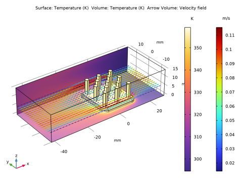
In the Settings window for 3D Plot Group, type Temperature and Fluid Flow, with Radiation in the Label text field.
2
In the Model Builder window, expand the Temperature and Fluid Flow, with Radiation node.
Fluid Flow
1
In the Model Builder window, expand the Results>With radiation>Temperature and Fluid Flow, with Radiation>Fluid Flow node, then click Fluid Flow.
2
In the Settings window for Arrow Volume, locate the Arrow Positioning section.
3
Find the x grid points subsection. In the Points text field, type 40.
4
Find the y grid points subsection. In the Points text field, type 20.
5
Find the z grid points subsection. From the Entry method list, choose Coordinates.
6
In the Coordinates text field, type 5.
Filter 1
1
In the Model Builder window, click Filter 1.
2
In the Settings window for Filter, locate the Element Selection section.
3
In the Logical expression for inclusion text field, type spf.U>0.25*nitf1.Uave.
4
In the Temperature and Fluid Flow, with Radiation toolbar, click  Plot.
The plot in the Graphics window should look like that in the figure below.