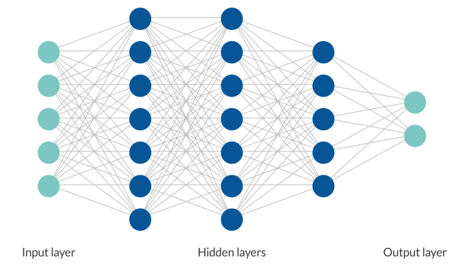
The Deep Neural Network function () provides training and validation using a deep neural network (DNN) for use with surrogate model training, for example. Deep neural networks form a class of machine learning algorithms similar to the artificial neural network and aims to mimic the information processing of the brain. DNNs have more than one hidden layer situated between the input and output layers.

Click the Train Model button ()) to train the deep neural network that you have specified from scratch. Click the Continue Training button (), when applicable, to continue the training from the current weights.

Click the Add button () under a list of layers to add a new layer. In the Type column, choose Dense (the default). In the Settings column, the following settings appear:

From the Activation list, specify an activation function, which defines how the weighted sum of the input is transformed into an output from a node or nodes in a layer of the network. The default activation is tanh, for a hyperbolic tangent function, which is an S-shaped function. You can also choose None for no activation function; ReLU for a rectified linear unit, an activation function defined as the positive part of its argument; ELU for an exponential linear unit; or Sigmoid for a sigmoid function. The default activation, tanh, is usually a good choice. ELU and ReLU are less smooth than the other functions, so avoid them if the trained function later needs to be differentiated. Choosing None is only useful for the last layer.

Use the Move Up (), Move Down (), and Delete () buttons and the fields under tables to edit the table contents. Or right-click a table cell and select Move Up, Move Down, or Delete.

From the Data source list, choose File (the default) or Result table.

If you chose File, then also specify these additional settings:

The File option supports data on the COMSOL spreadsheet format.

If you chose to Result table, then choose an available result table from the Result table list.

The Ignore NaN/Inf data points check box is selected by default to ignore data points that are NaN (Not-a-Number) or Inf (infinity). Clear it if desired.

For all types except Ignored column, specify a Scaling: Scale to [0,1] to scale it to values between 0 and 1 (the default) or No for no scaling. You can also edit the name of the function or argument in the Name field underneath and also provide a unit in the Unit field.

From the Method list, choose Adam (the default) or SGD. Adam is an adaptive learning rate optimization algorithm that is designed specifically for training deep neural networks. SGD is a stochastic gradient descent method with momentum. SGD with momentum is a method that helps accelerate gradient vectors in the right directions, leading to faster convergence.

In the Learning rate field, enter a suitable value for the learning rate (default: 1·10−3). The the learning rate is a configurable hyperparameter used in the training of DNNs. It typically has a small positive value.

The Momentum field (default: 0; that is, no momentum) is only available when Method is set to SGD. The momentum is a nonnegative number; a suitable number could be somewhere in the range of 0.9–0.99.

In the Weight decay field (default: 0; no extra penalization of the loss function’s complexity), enter a small nonnegative number to penalize complexity by adding the squares of all the parameters to the loss function, limiting the size of that term by multiplying it with the weight decay.

In the Batch size field (default: 512) enter a positive integer for the batch size, which defines the number of samples that will be propagated through the DNN. A batch size smaller than the total number of samples reduced the memory use and can provide faster training of the DNN. A too small batch size can also lead to more noise in the optimization. Defining what is too small depends on the problem.

From the Loss function list, choose Root-mean-square error (the default) or Mean absolute error. The loss function is used to estimate the error of a set of weights in a DNN. The default is to use a root-mean-square (RMS) error, which is calculated as the square root of the mean of the squared differences between the predicted and actual values. The result is always positive regardless of the sign of the predicted and actual values. The mean absolute error (MAE) is a measure of errors between paired observations expressing the same phenomenon and has similar properties. A difference is that with RMS, the errors are squared before they are averaged, which can give more weight to large errors and make RMS the better choice if large errors are particularly undesirable.

DNN algorithms are stochastic. This means that they make use of randomness, such as initializing to random weights; the same network trained can therefore produce different results using the same data. For the random seed, from the Random seed list choose Fixed (the default), which you enter into the Random seed field (default: 0), or choose Current computer time to pick the random seed from the current computer time.

Under Stop condition, specify a value in the Number of epochs field (default: 1000). The number of epochs is a hyperparameter that defines the number times that the learning algorithm will work through the entire training dataset. In each epoch all input data is processed once. The right number of epochs depends on the inherent perplexity (or complexity) of your dataset. If you find that the model is still improving after all epochs complete, try again with a higher value. If you find that the model stopped improving way before the final epoch, try again with a lower value as you may be overtraining the DNN. The training will use the weights that gave the smallest error on the validation data. This prevents using overtrained weights, so the main reason to not specify a too large number of epochs value is that it makes the training take more time than needed.

Under Validation data, you specify a number of settings for the validation data used for the DNN.

From the Validation data list, choose the type of validation data:

If you have generated training and validation data separately, you can either import the validation data to a table and use Separate table or store the validation data last in the same file as the training data and use Last part of data values. The Every N:th data value type is only good if the data file has been generated in a way that makes sure every N:th value gives a good sample of data points. In other cases, using Random sample of data is best.

From the Function name list, choose the function values to plot.

The plot parameters are set automatically when the function is trained, from the lower bound and upper bound settings for the corresponding probability distribution. It is possible to change the values manually after training. Then use the table below to set the range for arguments in preview plots. For each argument, enter a Lower limit, and an Upper limit in the Plot Parameters table. Use the check boxes in the Plot column to control which arguments to use in the plot (you can select a maximum of three arguments). If you clear a check box, a constant value, taken from the argument’s lower limit, is used. Constant arguments do no use an axis in the plot. These values and settings are used when you click the Plot button () or the Create Plot button () at the top of the Settings window.