The algebraic yPlus turbulence model is an algebraic turbulence model based on the distance to the nearest wall. The model is based on Prandtl’s mixing-length theory and is suitable for internal flows. It is less mesh sensitive than transport-equation models like Spalart–Allmaras or the
k-
ε model. In what follows, let
y be the coordinate normal to the wall, and
U the velocity parallel to the wall. Using a mixing length formulation, the balance for the shear stress in the wall layer may be approximated as
where y+ = yuτ/ν,
u+ = U/uτ and

is the friction velocity. Close to the wall, the mixing length must be zero such that
u+ = y+, and far away from the wall,

such that
u+ = (1/κ)log
(y+) + B. To obtain the correct behavior, the mixing length is chosen to be
where y* is to be determined. Inserting
Equation 3-68 into
Equation 3-67
This requires the local value of y+, which is obtained from the Reynolds number
The nonlinear algebraic Equation 3-72 has to be solved at each node point to evaluate the effective viscosity from
Equation 3-71. The local Reynolds number Re
= Uy/ν is formed with the local absolute value of the velocity and the distance to the nearest wall. This implicitly assumes that the main flow direction is parallel to the wall.
The wall distance, y is provided by a mathematical Wall Distance interface that is included when using the Algebraic yPlus model. The solution to the wall distance equation is controlled using the parameter
lref. The distance to objects larger than
lref is represented accurately, while objects smaller than
lref are effectively diminished by appearing to be farther away than they actually are. This is a desirable feature in turbulence modeling since small objects would get too large an impact on the solution if the wall distance were measured exactly.
The Algebraic yPlus turbulence model is consistent with a no slip boundary condition, that is u = 0. Since the turbulence model is algebraic, no additional boundary condition is needed. This boundary conditions is applied for
Wall Treatment equal to
Low Re.
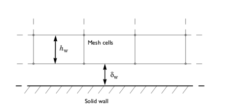
The default boundary treatment for Algebraic yPlus is the Automatic wall treatment. The automatic wall treatment assumes that there is a small gap,
δw =
hw/2, between the computational domain and the physical wall. Here,
hw is the height of the mesh cell adjacent to the wall. wall (see
Figure 3-7).

The automatic wall treatment tends to the low-Reynolds-number formulation when hw tends to zero, and it becomes a wall function formulation when the resolution in viscous units,
Δw+ increases. The resolution in viscous units is available as a postprocessing variable,
Delta_wPlus.
See also Wall for boundary condition details.
