Light that propagates through a dielectric waveguide has most of the power concentrated within the central core of the waveguide. Outside the waveguide core, in the cladding, the electric field decays exponentially with the distance from the core. However, if you put another waveguide core close to the first waveguide (see Figure 14), that second waveguide will perturb the mode of the first waveguide (and vice versa). Thus, instead of having two modes with the same effective index, one localized in the first waveguide and the second mode in the second waveguide, the modes and their respective effective indices split and you get a symmetric supermode (see
Figure 14 and
Figure 16 below), with an effective index that is slightly larger than the effective index of the unperturbed waveguide mode, and an antisymmetric supermode (see
Figure 15 and
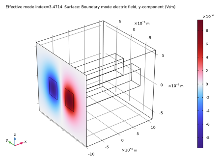
Figure 17), with an effective index that is slightly lower than the effective index of the unperturbed waveguide mode.
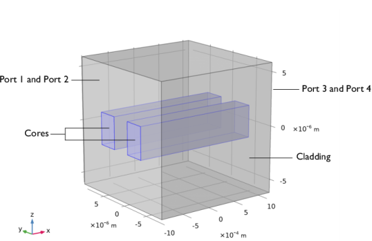
The directional coupler, as shown in Figure 13, consists of two waveguide cores embedded in a cladding material. The cladding material is GaAs, with ion-implanted GaAs for the waveguide cores. The structure is modeled after
Ref. 1.
The core cross section is square, with a side length of 3 μm. The two waveguides are separated 3
μm. The length of the waveguide structure is 2 mm. Thus, given the narrow cross section compared to the length, it is advantageous to use a view that does not preserve the aspect ratio for the geometry.
The model uses two numeric ports per input and exit boundary (see Figure 13). The two ports define the lowest symmetric and antisymmetric modes of the waveguide structure.
where ET,target is the tangential target electric field and
ci and
ET0,i are the expansion coefficients and the tangential non-normalized electric mode fields for mode
i, respectively. Taking the cross product with the complex conjugate of the tangential magnetic mode field for mode
j, multiplying with the port normal and integrating over the port boundary, we get
where Pj is the mode power for mode
j. Thus, the expansion coefficients are given by the overlap integral
where Pin,i is the specified input power for mode
i and
θin,i is the corresponding specified mode phase.
Equation 6 and
Equation 7 can now be used for specifying the input power and mode phase for the two exciting ports.
Figure 14 to
Figure 17 show the results of the initial boundary mode analysis. The first two modes (those with the largest effective mode index) are both symmetric.
Figure 14 shows the first mode. This mode has the transverse polarization component along the
z direction. The second mode, shown in
Figure 16, has transverse polarization along the
y direction.

Figure 15 and
Figure 17 show the antisymmetric modes. Those have effective indices that are slightly smaller than those of the symmetric modes.
Figure 15 shows the mode for
z-polarization and
Figure 17 shows the mode for
y-polarization.
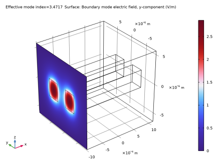
Figure 18 shows how the electric field increases in the receiving waveguide and decreases in the exciting waveguide. If the waveguide had been longer, the waves would switch back and forth between the waveguides.
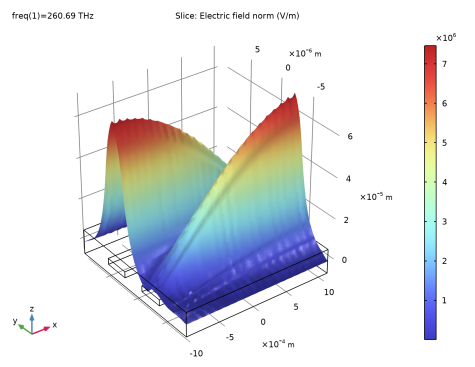
Figure 19 shows the result, when there is a
π phase difference between the fields of the exciting ports. In this case, the superposition of the two modes results in excitation of the other waveguides (as compared to the case in
Figure 18).
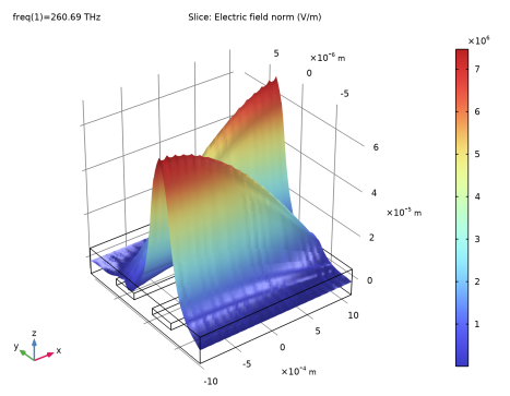
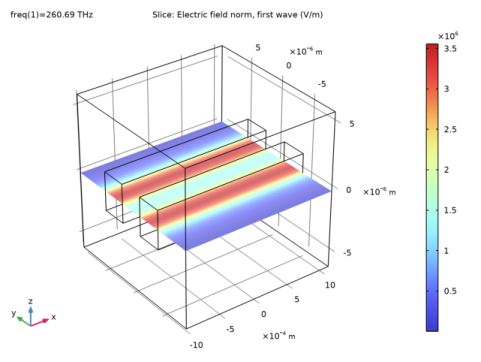
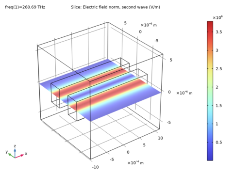
Figure 20 and
Figure 21 display the amplitudes of the first and second wave, respectively, when the bidirectional formulation is used. As expected, the amplitudes are almost constant.
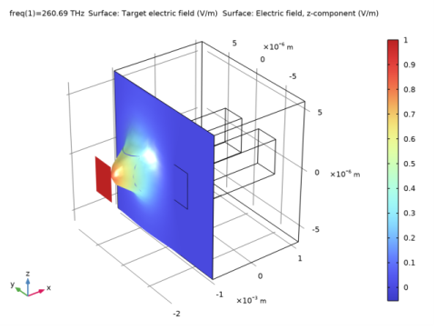
Figure 22 shows that the input field approximates the square target field, centered on the left waveguide, when the input power and the mode phase for the two exciting ports are calculated using an overlap integral between the target field and the mode field (c.f.
Equation 6 and
Equation 7).
 ,
, ,
, .
.