A prerequisite for setting up the mechanical contact problem is to define the contact search between the source boundary and the destination boundary. The purpose of the search is to detect points on the contacting boundaries that are in contact or may come in contact, and also to map quantities between such points. This part of the contact problem is defined in the Contact Pair that sets up relevant variables and operators to map quantities between the selected source and destination boundaries. In COMSOL Multiphysics, the contact search is made using a ray-tracing strategy as depicted in Figure 3-34. For mechanical contact, most variables and equations are formulated on the destination boundary. Hence, the typical mapping of interest here is from the source boundary to the destination boundary, however, it is possible to map quantities in the opposite direction as well.

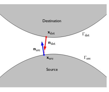
For each point xdst in the spatial frame on the destination boundary Γdst, the closest point xsrc in the spatial frame on the source boundary Γsrc in the direction of the destination spatial normal ndst is sought. Such a mapping can be described through an operator map(E, x), where E is some generic quantity or expression, and x is the point to which E is mapped. Using this mapping operator, the coordinates of the mapped point on Γsrc is

where x is the spatial coordinates that parameterize Γsrc. For brevity, the second argument of the mapping operator is omitted in the following and it should be understood that the mapping occurs to a point xdst on Γdst if nothing else is specified.

An important quantity for contact mechanics is the gap function ggeom(x) defined as the geometric distance between the source and the destination boundary. Note that ggeom(x) is not necessarily the closest distance between the two boundaries. Using the mapping operator, the gap distance at xdst is defined as

With the above definitions, a positive gap infers that there is a geometrical separation between the points, while a negative gap that there is an overclosure. Apart from the mapping operator, the Contact Pair also defines a dedicated variable for the gap function with the name geomgap_dst_<pair_tag>.

For the mechanical contact problem, it is additionally possible to define a physical offset from the geometric source and destination boundary. This means that the physical gap function gn(x) and geometrical gap function do not necessarily coincide. The physical gap distance including offsets at xdst is defined as

where doffset,s and doffset,d is the offset from the source and destination boundary, respectively. Each offset variable can vary along the geometry, and may also vary in time (or by the parameter value when using the continuation solver). The correction of the source side offset is necessary since the normal of xsrc, nsrc = map(n), is not necessarily pointing towards xdst as illustrated in Figure 3-34. When the geometric surfaces are in contact, the normals will be exactly opposite such that nsrc = -ndst.

In some cases, the discretization of the geometry, especially at curved boundaries, will give small irregularities in the gap function. You can then choose to adjust the physical gap by removing the geometric gap computed in the initial configuration, ginit, smaller than the tolerance Δgap. In this case, the physical gap function at xdst is

For problems including friction or adhesion, it is also necessary to know the tangential movement, or slip, between the source and destination boundary. The rate of the relative slip vector gt between the two boundaries at xdst is defined as

where X is the material coordinates, and F is the deformation gradient that contains information about the local rotation and stretch. Note that the mapping is made between points in the spatial frame as clarified in the equation. Both quantities are mapped from the source to the destination boundary. Constitutive models for the mechanical problem are typically formulated on an incremental form. COMSOL Multiphysics applies a backward Euler approximation to Equation 3-175 so that the incremental slip at xdst is

where Xsrc,old is the mapped material coordinates at the previous increment.

When a Contact node is added to a Shell, Layered Shell, or Membrane interface, the material and spatial frames used in the contact mapping are adjusted to account for the thickness of the structural element by considering the physical position of its top and bottom surface relative to the geometric boundary. This also applies to boundaries that intersect the selection of a Thin Layer node in the Solid Mechanics interface. For example, the contact material coordinates Xcnt and the spatial coordinates xcnt in a Contact node added in the Shell interface are defined as

where ndst is to be interpreted as the normal of the contact boundary. For the Shell interface, the direction of ndst coincides with the normal of the geometric boundary, but so is not always the case. This applies to nsrc as well. Note also the that mapping is made between the modified spatial coordinates. Similar corrections are also made for other quantities such as the incremental slip Δgt where the Xcnt is used instead of X. The same concept is used for other cases where the contact boundary does not coincide with the geometric boundary, but the definition of Xcnt and xcnt may differ.