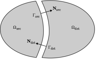
The Continuity node is a way to connect disconnected parts of an assembly by adding constraints or equations on a shared boundary. Consider a problem with two domains
Ωsrc and
Ωdst with a fully or partially shared boundary
Γint such that

, as is schematically shown in
Figure 3-33.
where Pi is the fist Piola-Kirchoff stress tensor,
Ti is the nominal traction, and
Ni is the normal vector in the material frame for the respective sides of the interface. The first condition represents the continuity of displacements and the second follows from the Newton’s third law. If the
Classical constraints method in the Continuity node is used, pointwise constraints are set up on
Γdst to enforce the continuity of displacements given by
Equation 3-171. This is accomplished with the help of the mapping operator
map(
E,
x) that is set up by the
Identity pair, where
E is some generic quantity to be mapped and
x is the point to which
E is mapped. Using this operator, the constraint equation is written as
where it is here implied that the mapping is made using material coordinates X, and that the mapping is made from
Γsrc to
Γdst. The above pointwise constraint implicitly enforces the condition given by
Equation 3-172. The above constraint equation can also be implemented as weak constraints by introducing Lagrange multipliers.
Another alternative is to use the Nitsche method, which was originally suggested by J. Nitsche in 1971 to weakly impose Dirichlet conditions without having to add Lagrange multipliers. To implement the continuity condition by the Nitsche method, one can, following for example
Ref. 4, start from the weak form of a generic boundary condition
where A(
u) is a flux-like operator and
B(
u) is a trace-like operator that can be seen as a conjugate pair, and
δ represents the test function. The next step is to reformulate these operators as
where c is a known quantity such as a prescribed displacement,
γ is a stabilization factor, and
θ is a parameter used to control the symmetry of the formulation. Inserting these reformulations of
A(
u) and
B(
u) into
Equation 3-173, after simplification, leads to the following weak contribution for implementing the Nitsche method for a generic boundary condition
To implement the continuity condition the unknowns A(
u),
B(
u), and
c has to be identified. Considering the continuity of displacements in
Equation 3-171, the displacement jump across the interface is defined as
and one can also realize that for continuity, c = 0. The Nitsche formulation of the continuity conditions then follows as
From the above weak equation several variants of the Nitsche formulation can then be set up. Firstly, it is possible to parameterize the integrals on both sides of the interface, or alternatively on either Γsrc or
Γdst only. The first option is less sensitive to the mesh on either side, but can be more expensive since it involves more mapping operations to evaluate. Secondly, the parameter
θ makes it possible to set up formulations with different properties and stability: