When solving, predefined plots containing the applied loads are generated. You can add them from the Add Predefined Plots window.
Figure 2-42 shows an example of such a plot. In this section, it is described in detail how you can work with these plots to fine-tune the visualization.
For each structural mechanics physics interface and dataset, a node group is generated under Results. Its name is
Applied Loads (<interfaceTag>). Within this node group, one plot group per type of load is created. The possible plot group names are listed in
Table 2-21.
|
|
|
|
|
|
|
Generated from Body Load, Gravity, Linearly Accelerated Frame, and Rotating Frame. The plot type depends on the geometrical dimension of the physics interface.
|
|
|
|
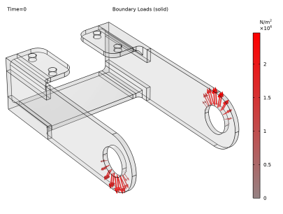
Generated from Boundary Load. Also, from Added Mass on a boundary combined with Gravity or Rotating Frame.
|
|
|
|
Generated from Face Load in Shell, Plate, and Membrane interfaces.
|
|
|
|
Generated from Face Load in Shell, Plate, and Membrane interfaces of nonzero moments are present.
|
|
|
|
Generated from Edge Load. Also, from Added Mass on an edge combined with Gravity or Rotating Frame.
|
|
|
|
Generated from Edge Load in Shell, Plate, and Beam interfaces if nonzero moments are present.
|
|
|
|
|
|
|
|
Generated from Point Load in Shell, Plate, and Beam interfaces if nonzero moments are present.
|
|
|
|
Generated from global features like Rigid Connector and Rigid Material, which have subnodes as Applied Load and Applied Moment. Such loads are a type of point load, but they are applied at a certain location in space, rather than at a point in the geometry.
|
|
|
|
Generated from Fluid Load in Pipe Mechanics interface.
|
|
|
|
Generated from Fluid Load in Pipe Mechanics interface.
|
Within a load group, the style of each load plot is inherited from the previous plot. The inheritance can be modified in the Inherit Style section. For example, clear the
Color check box to enable different color schemes for different loads and the
Color and data range to allow different ranges of the color legends.
In order not to hide any load arrows, the default is to use a transparent representation of the geometry. This is obtained through the extra surface plot Gray Surfaces together with a
Transparency subnode. This plot adds a uniform gray surface on each boundary of the geometry. The effect is shown in
Figure 2-42. If you disable the
Gray Surfaces plot, the structure will have a wireframe outline only. You can modify the transparency level in the
Transparency subnode, or delete the node completely. You can, furthermore, add a
Selection subnode to the
Gray Surfaces node to modify on which boundaries to plot the gray surface.
The Gray Surfaces plot is only generated for physics that use a 2D or 3D representation of the geometry.
You can change the attachment of the arrow by changing the setting of Arrow base in the
Coloring and Style section. The default is in most cases to place the tail on the geometry. One exception is, for example, a pressure boundary load for which the head of the arrow is placed at the geometry.
For distributed fields, the default is to place one arrow at the center of each element, element face, or element edge. If the density of arrows is not appropriate, you can modify the settings in the Arrow Positioning section. For example, change
Placement to
Mesh nodes to place an arrow in each point of the of the linear mesh, or set it to
Uniform to specify an arbitrary number of arrows to be plotted.
The color scheme of the arrow plots is controlled in a Color Expression subnode. The default color table is a
Gradient going from red to black. You can change this in the
Coloring list. By selecting
Color table, the color table is automatically set to
Spectrum. This color table can be useful for a clear visualization of the applied loads, when, for example, the magnitude varies significantly between load features.
By default, the load plots are presented in the initial configuration of the model. However, when applicable, a Deformation subnode is added to each plot, but with the
Scale factor set to zero. Modify the scale factor to view the loads in a deformed state. Note that when multiple load plots exist in a plot group, the scale factor is by default inherited from the first plot. The exception is the
Gray Surfaces plot, where the scale factor is set independently of the other plots.
When the analysis includes geometric nonlinearities, the Scale factor is by default set to one. Hence, the loads are presented in the deformed configuration for such cases.