Stress Linearization


	The information about stress linearization is applicable if your license includes the Structural Mechanics Module.

Stress linearization is a procedure in which the stress distribution along a line through the thickness in a solid is approximated with an equivalent linear stress distribution, similar to what would be the result of an analysis using shell theory. The line is commonly referred to a stress classification line, SCL. This type of evaluation is common in the analysis of pressure vessels. It is also useful for the design of reinforcements for concrete structures and for fatigue analysis of welds.

To perform a stress linearization, you add one Stress Linearization node for each SCL.

Orientation of Stress Components

The stresses along the SCL are represented in a local orthonormal coordinate system, x1-x2-x3. The x1 direction is oriented along the SCL, so it is mainly the stresses in the second and third directions that are of interest.

•

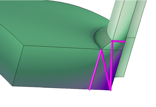
In 3D, you must specify the x2 direction and thus implicitly the x3 direction. You specify the orientation either by selecting a point in the x1-x2 plane or by defining an orientation vector in an approximate x2 direction. In either case, the actual x2 direction is chosen so that it is perpendicular to the SCL and lies in the plane you have specified. The x3 orientation is then taken as perpendicular to x1 and x2. As long as you are only interested in a stress intensity, the choice of orientation is arbitrary.

•

In 2D, the x3 direction is the out-of-plane direction, and the x2 direction is perpendicular to the SCL in the XY-plane.

•

In 2D axial symmetry, the x3 direction is the azimuthal direction, and the x2 direction is perpendicular to the SCL in the RZ-plane.

Creating the Stress Classification Line

The most straightforward way to create an SCL is to include it in the geometry, and then select it in a node. This corresponds to using the linearization type where the SCL is defined by .

Figure 2-35: Four stress classification lines in a transition region at a pressure vessel nozzle.

There are, however, some situations where this direct approach is less convenient:

•

When the introduction of the SCL in the geometry must be done after the analysis, since the locations of critical regions were not obvious when setting up the initial analysis. It is of course possible to add new edges and rerun the analysis, but this may not be a good solution if the analysis time is long.

•

When the introduction of the edges for the SCL makes the meshing more difficult. It may, for example, not be possible to use swept meshes anymore, or the mesh quality is reduced in critical regions.

In the two above cases an alternative is to define an SCL that is not included in the geometry by connecting two arbitrary points with a straight line. This corresponds to using the linearization type where the SCL is defined by . The introduction of the SCL will in this case not make it necessary to update the geometry and rerun the analysis. Since the SCL is disconnected from the geometry and mesh, this option will also make meshing easier. The downside is then the you cannot control the mesh quality along the SCL.

In some cases it is difficult to a priori determine where to create the SCL or the critical location may change depending on, for example, loading conditions or time. For such cases, it is also possible to define it in a distributed manner such that an infinite number of SCLs are created in a domain. The starting point of the SCLs are given by a boundary selection, and they extend along the normals of the boundary through the selected domains. This corresponds to using the linearization type.

Studies and Solutions

Stress linearization is a pure postprocessing operation. The node will only create a number of variables, which can be evaluated under . It is thus possible to add such nodes after the main analysis has been performed. In order to make the new variables available for postprocessing, you must then run an .

Results

When you have included one or more nodes in a model, a number of datasets and an extra predefined plot are generated.

One edge dataset is created for each SCL. These datasets are named Linearization Line <n>, where n is an integer number.

Figure 2-36: Generated datasets in a model with five SCL.

The plot contains graphs for the 22 component of the actual stress, the membrane stress, and the linearized stress. The first dataset is selected. By changing edge dataset in the plot group, you can easily move between the different stress classification lines.

Figure 2-37: Plot along a stress classification line.

For the linearization type, the created dataset corresponds to a single SCL in selected domain. The starting point is specified in the section of the feature, and must lie on the selected boundaries. The endpoint is computed internally such that the cut line extends through the selected domains along the boundary normal of the point.

Variable Names

Each node adds a number of variables. Many of these variables exist with two different scopes, physics scope and feature scope. The physics scope is the name of the physics interface, having the default value ‘solid’. The feature scope contains also the tag of the node, for example, ‘sl1’.

As an example, the variable solid.Sm22 and the variable solid.sl1.Sm22 have the same value. The variables with physics scope make it more convenient to create expressions using postprocessing. You could, for example, make a line plot of solid.sb22 and get all edges having a stress linearization colored by their individual results.

Table 2-19: Variables for Stress Linearization
Variable	Description	Variable in theory Section	Comment	Scope
Sllsij	Stress tensor in local coordinate system	σij	ij = 11, 12, 13, 22, 23, 33	Physics, Feature
Smij	Membrane stress	σm,ij	ij = 11, 12, 13, 22, 23, 33	Physics, Feature
Sbmaxij	Maximum bending stress	σb(max),ij	ij = 11, 12, 13, 22, 23, 33	Feature
Sbij	Bending Stress	σb,ij	ij = 11, 12, 13, 22, 23, 33	Physics, Feature
Smbij	Membrane + bending stress	σmb,ij	ij = 11, 12, 13, 22, 23, 33	Physics, Feature
Spsij	Peak stress, starting point	σp(start),ij	ij = 11, 12, 13, 22, 23, 33	Feature
Speij	Peak stress, starting point	σb(end),ij	ij = 11, 12, 13, 22, 23, 33	Feature
SIm	Stress intensity, membrane	σint		Physics, Feature
SImbs	Stress intensity, membrane + bending, starting point	σint		Feature
SImbe	Stress intensity, membrane + bending, endpoint	σint		Feature
SImb	Stress intensity, membrane + bending,		max(SImbs, SImbe)	Physics, Feature
Nij	Local in-plane force	Nij	ij = 22, 23, 33	Feature
Mij	Local bending moment	Mij	ij = 22, 23, 33	Feature
Qi	Local out-of-plane shear force		i = 2, 3	Feature
lengthtot	Length of SCL	L		Feature
arclength	Coordinate along SCL	X1		Feature


	Stress Linearization in the Structural Mechanics Theory Chapter.