Buckling Analysis

A linearized buckling analysis can be used for estimating the critical load at which a structure becomes unstable. This is a predefined study type that consists of two study steps: An initial step in which a unit load is applied to the structure, and a second step in which an eigenvalue problem is solved for the critical buckling load.

The idea behind this type of analysis can be described in the following way:

Consider the equation system to be solved for a stationary load f, in case of geometric nonlinearity;

Here the total stiffness matrix, K, depends in the solution, since the problem is nonlinear. It has been split into a linear part, KL, and a nonlinear contribution, KNL.

In a first-order approximation, KNL is proportional to the stress in the structure and thus to the external load. If the linear problem is solved first for an arbitrary initial load level f0,

(2-38)

then the nonlinear problem can be approximated as

where λ is called the load multiplier.

An instability is reached when this system of equations becomes singular, so that the displacements tend to infinity. The value of the load at which this instability occurs can be determined by, in a second study step, solving an eigenvalue problem for the load multiplier λ.

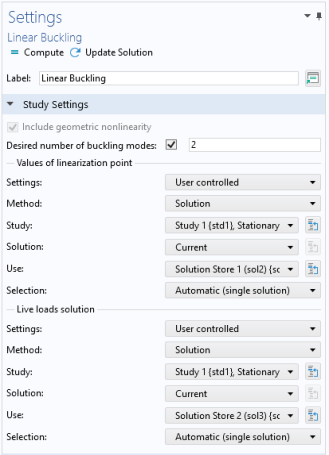
COMSOL reports a critical load factor, which is the value of λ at which the structure becomes unstable. The corresponding deformation is the shape of the structure in its buckled state.

The level of the initial load used is immaterial since a linear problem is solved. If the initial load actually was larger than the buckling load, then the critical value of λ is smaller than 1. It is also possible that the computed value of λ is negative. This signifies that a reversed load will give the critical case.

Live and Dead Loads

In some situations, not all loads that act on the structure can vary, and you may want to compute the critical load factor only with respect to the uncertain (‘live’) load. For example, gravity is often treated as a ‘dead’ load. The dead loads do, however, affect the stress distribution in the structure, so they cannot be completely ignored. Using the same terminology as above,

Here, the superscripts ‘d’ and ‘l’, stands for live and dead loads, respectively. By solving two problems, one with the live loads, and one with the dead loads, it is possible to separate their effects:

Now, the following eigenvalue problem is solved to determine the critical load factor:

For any load feature, you can specify that is a dead load by selecting the check box in the section.

To perform a buckling analysis including both live and dead loads, you need three study steps: two stationary steps, and the linear buckling study step.

In the first study step, you solve for the dead loads only. Disable any live loads in the solver.

In the second study step, you solve for all loads; the live loads with an arbitrary scaling factor plus the dead loads.

Finally, in settings for the study step, you need to point to these two solutions as point and , respectively.

Figure 2-32: Selecting the solutions for a buckling analysis with live and dead loads.

Geometric Nonlinearity

Sometimes, the preload case requires a geometrically nonlinear analysis in order to produce the correct state. This means that it is no longer solved using the linear set of equations given by Equation 2-38, but rather

(2-39)

The assumption for the buckling analysis is still that KNL is proportional to the external load, even though this may be disputable for a strongly nonlinear case. KNL is based on the stresses, which must be computed in the same way for both cases, that is, under the same assumption about geometric nonlinearity. The effect is that the stiffness matrix at the linearization point includes the nonlinear part from Equation 2-39, and the eigenvalue problem is reformulated as

Follower Loads

Loads that depend on the deformation are called follower loads. An example of this is a pressure load, since the orientation of the load will depend on surface deformation. Such loads contribute to the stiffness matrix, and can thus affect the buckling load. As a default, all loads in the structural mechanics interfaces are multiplied by the load factor λ in a linear buckling study step.


	If the computation of the predeformation requires a geometrically nonlinear analysis, then geometric nonlinearity must be used also in the Linear Buckling study step. In this case, it must be assumed that the critical load factor λ is significantly larger than 1.

•

Be aware that for some structures, the true buckling load can be significantly smaller than what is computed using a linearized analysis. This phenomenon is sometimes called imperfection sensitivity. Small deviations from the theoretical geometrical shape can then have a large impact on the actual buckling load. This is especially important for curved shells.

•

For a structure that exhibits axial symmetry in the geometry, constraints, and loads, the critical buckling mode shape can still be nonaxisymmetric. A full 3D model should always be used when computing buckling loads.

•

It must always be checked that allowable stresses are not exceeded before the buckling load is reached.

•

Studies and Solvers and Linear Buckling in the COMSOL Multiphysics Reference Manual

•

Linear Buckling in the theory section of the Structural Mechanics Module User’s Guide

•

Bracket — Linear Buckling Analysis: Application Library path

•

Buckling Analysis of a Truss Tower: Application Library path