The Layered Shell Interface

The interface (

), found under the branch (

) when adding a physics interface, is used to model layered structural shells on 3D boundaries. Shells are thin flat or curved structures, having significant bending stiffness.

The Layered Shell interface is applicable for thick and moderately thin shells. The formulation resembles that of a stack of fully 3D solid mechanics models, so all stress components, including interlaminar shear stresses can be resolved. For very thin shells this formulation tends to become numerically ill-behaved, and it is then better to use the Shell interface with the model.

The Linear Elastic Material is the default material model. With the Nonlinear Structural Materials Module, the physics interface is extended with more material models, like hyperelasticity, plasticity, creep, and viscoplasticity.

When this interface is added, these default nodes are also added to the — , (a boundary condition where edges are free, with no loads or constraints), and . Then, from the toolbar, add other nodes that implement, for example, boundary conditions. You can also right-click to select physics features from the context menu.

The Layered Shell interface is only available with the Composite Materials Module (see https://www.comsol.com/products/specifications/).

The is the default physics interface name.

The is used primarily as a scope prefix for variables defined by the physics interface. Refer to such physics interface variables in expressions using the pattern <name>.<variable_name>. In order to distinguish between variables belonging to different physics interfaces, the name string must be unique. Only letters, numbers, and underscores (_) are permitted in the field. The first character must be a letter.

The default (for the first physics interface in the model) is lshell.

Here you select on which layers in a layered material that the physics interface should be active. By default, the check box is selected. This means that all layers in all layered materials on the selected boundaries are used.

If you deselect the check box, you can select individual layers within a single layered material. This is a seldom used option, since it means that the physics interface is restricted to the boundaries on which a specific layered material is defined.

	For a general description of layer selections, see The Shell Properties and Interface Selection Sections.

From the list, select (the default) or . Use to treat the dynamic behavior as quasistatic (with no mass effects; that is, no second-order time derivatives). Selecting this option gives a more efficient solution for problems where the variation in time is slow when compared to the natural frequencies of the system. The default solver for the time stepping is changed from Generalized alpha to BDF when is selected.

For problems with creep, and sometimes viscoelasticity, the problem can be considered as quasistatic. This is also the case when the time dependence exists only in some other physics, like a transient heat transfer problem causing thermal strains.

A fold-line is an edge where the boundaries that meet do not have a continuous orientation of the normal vector. Along fold lines, the degrees of freedom are in general not continuous, but rather connected by a set of constraints.

Select a — or . The full fold-line constraint formulation is accurate, consistent with the degrees of freedom, and does not produce any stress singularities near the fold-lines. However, it is computationally expensive, and leads to a nonlinear problem, even in an otherwise linear model. On the other hand, the simplified fold-line constraint formulation assumes that thin shell kinematics can be used. It is computationally more efficient, does not force the problem to be nonlinear, and works very well for thin or moderately thick shells.

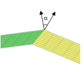
The fold-line limit angle α is the smallest angle between the normals of two boundaries that makes their intersection to be treated as a fold line. The normal to the layered shell is discontinuous along a fold-line. Enter a value or expression in the α field. The default value is 0.05 radians (approximately 3°). The value must be larger than 0, and less than π/2, but angles larger than a few degrees are not usually meaningful.

	See Fold-Line Connection for the theory of fold line constraints in layered shell.

Enter a number between -1 and 1 for the Z. The value can be changed from −1 (downside) to +1 (upside). The default is +1. A value of 0 means the midsurface of the layered shell. This is the default position for stress and strain evaluation during the results analysis.

To display this section, click the button (

) and select in the dialog box. Normally these settings do not need to be changed.

You can chose how to group in the solver nodes the extra ODE variables added by some features.

Select the check box to group in the solver node the variables added by the Rigid Connector and Rigid Connector, Interface features.

Select the check box to group in the solver node the variables added by the Attachment feature.

The selection made in the section can be overridden by the settings in the section of the Rigid Connector, Rigid Connector, Interface, or Attachment features.

In the Layered Shell interface you can choose not only the order of the discretization, but also the type of shape functions: Lagrange or serendipity. For highly distorted elements, Lagrange shape functions provide better accuracy than serendipity shape functions of the same order. The serendipity shape functions will however give significant reductions of the model size for a given mesh containing hexahedral, prism, or quadrilateral elements. The default is to use shape functions for the .

The order of the discretization is used not only in the reference surface but also in the thickness direction. It is possible to choose different order of discretization in the reference surface and in the thickness direction.

	See Discretization for the details on discretization order for a layered shell.

The physics interface uses the global spatial components of the u as dependent variables. The default names for the components are (u, v, w).

Since the Layered Shell Interface uses a discretization also in the thickness direction, the degrees of freedom are allocated not only in the plane of the shell, but also in that direction.

You can change both the field name and the individual component names. If a new field name coincides with the name of another displacement field, the two fields (and the interfaces which define them) share degrees of freedom and dependent variable component names.

A new field name must not coincide with the name of a field of another type (that is, it must contain a displacement field), or with a component name belonging to some other field. Component names must be unique within a model except when two interfaces share a common field name.