The Electromagnetic Waves, Frequency Domain (emw) interface () is used to solve for time-harmonic electromagnetic field distributions. It is found under the Radio Frequency branch () when adding a physics interface.

For this physics interface, the maximum mesh element size should be limited to a fraction of the wavelength. The domain size that can be simulated thus scales with the amount of available computer memory and the wavelength. The physics interface supports the Frequency Domain, Eigenfrequency, Mode Analysis, and Boundary Mode Analysis study types. The Frequency Domain study type is used for source driven simulations for a single frequency or a sequence of frequencies. The Eigenfrequency study type is used to find resonance frequencies and their associated eigenmodes in resonant cavities.

When this physics interface is added, these default nodes are also added to the Model Builder — Wave Equation, Electric, Perfect Electric Conductor, and Initial Values. Then, from the Physics toolbar, add other nodes that implement, for example, boundary conditions. You can also right-click Electromagnetic Waves, Frequency Domain to select physics features from the context menu.

The physics-controlled mesh is controlled from the Settings window for the Mesh node (if the Sequence type is Physics-controlled mesh). In the table in the Physics-Controlled Mesh section, find the physics interface in the Contributor column and select or clear the check box in the Use column on the same row for enabling (the default) or disabling contributions from the physics interface to the physics-controlled mesh.

When the Use check box for the physics interface is selected, this invokes a parameter for the maximum mesh element size in free space. The physics-controlled mesh automatically scales the maximum mesh element size as the wavelength changes in different dielectric and magnetic regions. If the model is configured by any periodic conditions, identical meshes are generated on each pair of periodic boundaries. Perfectly matched layers are built with a structured mesh, specifically, a swept mesh in 3D and a mapped mesh in 2D.

When the Use check box is selected for the physics interface, in the section for the physics interface below the table, choose one of the four options for the Maximum mesh element size control parameter — From study (the default), User defined, Frequency, or Wavelength. When From study is selected, 1/8 in 2D or 1/5 in 3D of the vacuum wavelength from the highest frequency defined in the study step is used for the maximum mesh element size. For the option User defined, enter a suitable Maximum element size in free space. For example, 1/5 of the vacuum wavelength or smaller. When Frequency is selected, enter the highest frequency intended to be used during the simulation. The maximum mesh element size in free space is 1/8 in 2D and 1/5 in 3D of the vacuum wavelength for the entered frequency. For the Wavelength option, enter the smallest vacuum wavelength intended to be used during the simulation. The maximum mesh element size in free space is 1/8 in 2D and 1/5 in 3D of the entered wavelength.

Furthermore, for Port and Lumped Port features, the maximum mesh element size can be slightly finer than what is discussed above.

When Resolve wave in lossy media is selected, the outer boundaries of lossy media domains are meshed with a maximum mesh element size in free space given by the minimum value of half a skin depth and 1/5 of the vacuum wavelength.

When Refine conductive edges is selected, the exterior edges of conductive boundaries, configured by perfect electric conductors, transition boundary, or layered transition boundary conditions, are meshed with a user-specified size. Adjust Angular tolerance (SI unit: rad) to include not only edges on flat surfaces but also curved surfaces. Choose Size type — Relative or User defined. For the option Relative, the mesh size on the selected edges is defined relative to the default maximum mesh size. On the other hand, when the option User defined is selected, the mesh size is set by user-defined value in the Size input field (SI unit: m).

When Add far-field boundary layers is selected, the far-field calculation boundaries adjacent to the selection of scattering boundary conditions or perfectly matched layers create a boundary layer mesh with a thickness of 1/40 to the default maximum mesh size.

The material property can be defined by a function, if the function use a single input argument, for example called freq, and this variable is also marked as a Frequency Model input in the material property group node where the function is used.

The Label is the default physics interface name.

The Name is used primarily as a scope prefix for variables defined by the physics interface. Refer to such physics interface variables in expressions using the pattern <name>.<variable_name>. In order to distinguish between variables belonging to different physics interfaces, the name string must be unique. Only letters, numbers, and underscores (_) are permitted in the Name field. The first character must be a letter.

The default Name (for the first physics interface in the model) is emw.

From the Formulation list, select whether to solve for the Full field (the default) or the Scattered field.

For Scattered field select a Background wave type according to the following table:

Enter the component expressions for the Background electric field Eb (SI unit: V/m). The entered expressions must be differentiable.

For Gaussian beam select the Gaussian beam type — Paraxial approximation (the default) or Plane wave expansion.

When selecting Paraxial approximation, the Gaussian beam background field is a solution to the paraxial wave equation, which is an approximation to the Helmholtz equation solved for by the Electromagnetic Waves, Frequency Domain (emw) interface. The approximation is valid for Gaussian beams that have a beam radius that is much larger than the wavelength. Since the paraxial Gaussian beam background field is an approximation to the Helmholtz equation, for tightly focused beams, you can get a nonzero scattered field solution, even if you do not have any scatterers. The option Plane wave expansion means that the electric field for the Gaussian beam is approximated by an expansion of the electric field into a number of plane waves. Since each plane wave is a solution to the Helmholtz equation, the plane wave expansion of the electric field is also a solution to the Helmholtz equation. Thus, this option can be used also for tightly focused Gaussian beams.

For Plane wave expansion select Wave vector distribution type — Automatic (the default) or User defined. For Automatic also check Allow evanescent waves, to include evanescent waves in the plane wave expansion. For User defined also enter values for the Wave vector count Nk (the default value is 13) and Maximum transverse wave number kt,max (SI unit: rad/m, default value is (2*(sqrt(2*log(10))))/emw.w0). Use an odd number for the Wave vector count Nk to make sure that a wave vector pointing in the main propagation direction is included in the plane-wave expansion. The Wave vector count Nk specifies the number of wave vectors that will be included per transverse dimension. So for 3D the total number of wave vectors will be Nk·Nk.

A plane wave expansion with a finite number of plane waves included will make the field periodic in the plane orthogonal to the main propagation direction. If the separation between the transverse wave vector components, given by 2kt,max/(Nk − 1), is too small, replicas of the Gaussian beam background field can appear. To avoid that, increase the value for the Wave vector count Nk.

For more information about the Gaussian beam theory, see Gaussian Beams as Background Fields and Input Fields.

The initial background wave is predefined as E0 = exp(−jkxx)z. This field is transformed by three successive rotations along the roll, pitch, and yaw angles, in that order. For a graphic representation of the initial background field and the definition of the three rotations compare with Figure 4-1 below.

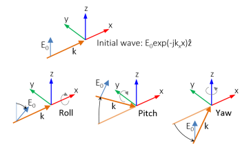
m is the azimuthal mode number (+1 or −1) varying depending on the Circular polarization type and Direction of propagation settings, and and are the unit vectors in the r and  directions, respectively.

Linearly polarized plane wave can be written as the sum of an infinite number of azimuthal modes in cylindrical coordinates. Thus, the Linearly polarized plane wave option available for 2D axisymmetric components enables fast simulation of scattering problem for body-of-revolution geometries. For a graphic representation of the initial background field and the definition of the three rotations have a look at Figure 4-2 below. To define a linearly polarized plane wave with arbitrary angle of incidence θ and polarization α:

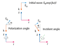
Select the Electric field components solved for — Three-component vector, Out-of-plane vector, or In-plane vector. Select:

This section is available for 2D and 2D axisymmetric components, when solving for Three-component vector or In-plane vector.

For 2D components, assign a wave vector component to the Out-of-plane wave number field. For 2D axisymmetric components, assign an integer constant or an integer parameter expression to the Azimuthal mode number field.

From the Methodology options list, select one of three solver configurations: Robust, Intermediate, or Fast (the default).

The settings of each methodology option are found in Solver Configurations and the subsidiary nodes.

Select the Use manual port sweep check box to enable the port sweep. When selected, this invokes a parametric sweep over the ports in addition to the frequency sweep already added. The generated lumped parameters are in the form of an S-parameter matrix.

For Use manual port sweep enter a Sweep parameter name to assign a specific name to the parameter that controls the port number solved for during the sweep. Before making the port sweep, the parameter must also have been added to the list of parameters in the Parameters section of the Parameters node under the Global Definitions node. This process can be automated by clicking the Configure Sweep Settings button. The Configure Sweep Settings button helps add a necessary port sweep parameter and a Parametric Sweep study step in the last study node. If there is already a Parametric Sweep study step, the sweep settings are adjusted for the port sweep.

Select Export Touchstone file and the S-parameters are subject to Touchstone file export. Click Browse to locate the file, or enter a file name and path. Select an Parameter format (value pair): Magnitude angle, Magnitude (dB) angle, or Real imaginary.

Enter a Reference impedance for Touchstone file export Zref (SI unit: Ω) that is used only for the header in the exported Touchstone file. The default is 50 Ω.

To display this section, click the Show More Options button () and select Advanced Physics Options in the Show More Options dialog box.

where E, r, Einc, Si, Ei, αi, n, and r0 are, respectively, the electric field on the port boundary, the position vector, the incident electric field, the expansion coefficient (or S-parameter), the mode field, the propagation constant for the mode, the normal vector, and a position on the port boundary.

Select Weak formulation (the default value) from the Port formulation list. In this formulation, the expansion coefficients (or S-parameters) are calculated by adding a scalar dependent variable for each coefficient. The S-parameter and the tangential electric field on the port boundary are solved for by adding the following weak expression for each port

where Js,i is the surface current density for the port

ET is the tangential electric field (the dependent variable) on the port boundary, δij is the Kronecker delta

Above, Hi is the magnetic mode field for the port, Ebnd is the expansion of the electric field on the port boundary in terms of the electric mode fields, Ei,

When Constraint-based is selected from the Port formulation list, the expansion coefficients (or S-parameters) are calculated by adding a scalar dependent variable for each coefficient and then adding a constraint to enforce the series expansion above.

The dependent variables (field variables) are for the Electric field E and its components (in the Electric field components fields). The name can be changed but the names of fields and dependent variables must be unique within a model.

Select the shape order for the Electric field dependent variable — Linear, Linear type 2, Quadratic (the default), Quadratic type 2, Cubic, or Cubic type 2. For more information about the Discretization section, see Settings for the Discretization Sections in the COMSOL Multiphysics Reference Manual.