Capacitively Coupled Plasmas
Capacitively coupled plasmas (CCP) represent a monumental challenge when it comes to numerical modeling for the following reasons. The main challenge is the overwhelming number of RF cycles before the plasma evolves to a time periodic steady state solution. COMSOL Multiphysics includes a special physics interface for such applications, which removes the need to solve the problem in the time domain, while still capturing all the nonlinearities involved in the discharge. This is the Plasma, Time Periodic interface.
Consider the following test problem, which roughly describes the evolution of a metastable species in a capacitively coupled plasma:
where u is representative of the amount of the metastable species. The first term on the right hand side represents the periodic production of the metastable in the plasma sheath, oscillating with period ω. The second term represents losses due to collisions with the background gas, and the third term losses due to collisions between the metastables.
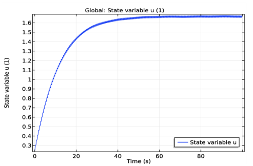
The evolution of the metastable density is shown in Figure 6-1. It takes close to 100 cycles before the value evolves to its periodic steady state solution. In many plasma reactors, it can be more like 50 or 100,000 RF cycles before this evolution is complete. Solving this in the time domain is computationally intractable.
Figure 6-1: Metastable density.
The above equation can be reformulated as a boundary value problem:
with periodic boundary conditions:
.
Solving this boundary value problem will immediately produce the solution during the period when the periodic steady state solution is reached. Thus, a time-dependent problem with enormous computational cost is replaced by a simple boundary value problem. This is the basic technique used in the Plasma, Time Periodic interface.
In order to facilitate the modeling process, the conversion to a boundary problem is accomplished by attaching an extra dimension to the reactor geometry. This forms a product space where the boundary value problem can be solved while leaving the model setup practically the same as when using the Plasma interface. All of the dependent variables may be solved for in the product space, and periodic boundary conditions are applied across the extra dimension. The Time Periodic study is used to solve this problem, but it is basically the equivalent of a Stationary study.
As well as reducing the computational burden, the technique also has the following advantages:
There are, of course a couple of downsides worth mentioning: