Boltzmann Equation, Two-Term Approximation
The Boltzmann equation describes the evolution of a distribution function, f, in six-dimensional phase space:
,
where v is the velocity coordinates, m is the electron mass, E is the electric field, is the velocity gradient operator, and C[f] is the rate of change in f due to collisions. To be able to solve the Boltzmann equation and thus compute the EEDF, drastic simplifications are necessary. It is assumed that the electric field and the collision probabilities are spatially uniform. The Boltzmann equation is then written in terms of spherical coordinates in the velocity space and f is expanded in spherical harmonics. The series is truncated after the second term and the so-called two-term approximation of f is
where f0 is the isotropic part of f, f1 is an anisotropic perturbation, v is the magnitude of the velocity, θ is the angle between the velocity and the field direction, and z is the position along this direction.
The last piece of simplification consists of separating the energy dependence of the EEDF from its time and space dependence. For steady state cases the separation can be formally written as
It is also possible to solve for the temporal evolution of F0 in which case
For both stationary and time-dependent cases F1 can be assumed to follow the electric field instantaneously or to be in the limit of an high frequency oscillating electric field. F0,1 is an energy distribution function that verifies the following normalization
Outside this section, for simplicity, f is used to refer to any EEDF. It is important to keep in mind that when the Boltzmann equation in the two term approximation is solved the EEDF is F0 as defined in this section.
Using the abovementioned approximations and after some manipulations, the Boltzmann equation can be written in the form of a 1D convection-diffusion-reaction equation
.
For more details, see Ref. 1 and Ref. 5. This equation is somewhat special because the source term is nonlocal and the convection and diffusion coefficients depend on the integral of the solution. The different terms, including the effects of electron-electron collisions, are presented below:
The following definitions apply
(3-1)
.
The approach presented until now is valid in situations where the electric field is constant on the time scale of the collisions (referred as the DC limit). For high-frequency oscillating electric fields, in conditions such that the characteristic frequency for energy transfer is much lower than the field frequency (referred to as the HF limit), the same approach can be used with the following modification for Q
where qw is the equivalent cross section for AC field oscillations
.
Here:
γ = (2q/me)1/2 (SI unit: C1/2/kg1/2)
me is the electron mass (SI unit: kg)
ε = (v/γ)2 is energy (SI unit: V)
σε is the total elastic collision cross section (SI unit: m2)
σm is the total momentum collision cross section (SI unit: m2)
q is the electron charge (SI unit: C)
ε0 is the permittivity of free space (SI unit: F/m)
T is the temperature of the background gas (SI unit: K)
kb is the Boltzmann constant (SI unit: J/K)
ne is the electron density (SI unit: 1/m3)
Nn is the background gas density (SI unit: 1/m3)
Λ is the Coulomb logarithm, and
M is the mass of the target species (SI unit: kg).
The source term, S represents energy loss due to inelastic collisions. Because the energy loss due to an inelastic collision is quantized, the source term is nonlocal in energy space. The source term can be decomposed into four parts where the following definitions apply:
where xk is the mole fraction of the target species for reaction k, σk is the collision cross section for reaction k, Δεk is the energy loss from collision k, and δ is the delta function at ε = 0. The term changes slightly when equal energy sharing is used:
.
Note the factor of 4 differs from the factor of 2 used in Ref. 1, as was later corrected in Ref. 4. The term, λ is a scalar-valued renormalization factor that ensures that the EEDF has the following property:
(3-2)
An ODE is implemented to solve for the value of λ such that 
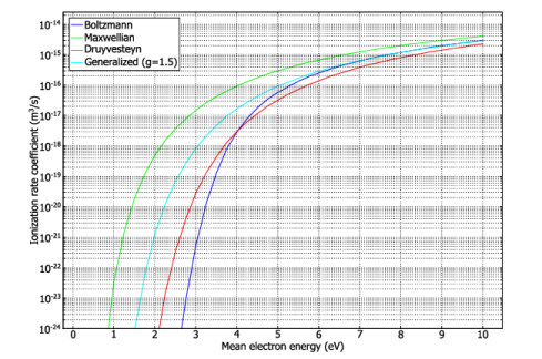
Equation 3-2 is satisfied. The rate coefficients are computed from the EEDF by way of the following integral:
The mean electron energy is defined by the integral
(3-3)
In order to set the mean electron energy to a specific setpoint, a second Lagrange multiplier is introduced to solve for the reduced electric field, such that Equation 3-3 is satisfied. The weak form of the constraint is:
where tilde denotes test function.
The reduced transport properties associated to a DC transport are computed using the following integrals
In the HF limit the real and imaginary part of the mobility are available and are used to computed the power absorbed by the electrons and the plasma conductivity
.
The power absorbed by the electrons from the electric field in the DC limit is given by
and in the HF limit by
.
The elastic power loss is defined as
.
The inelastic power loss is defined as
.
The growth power associated with the apparent energy loss due to electrons appearing and disappearing in ionization and attachment is given by:
,
where νion and ηatt are the total ionization frequency and the total attachment frequency defined as:
.
Note that the solution of the Boltzmann equation in this approach should verify
.
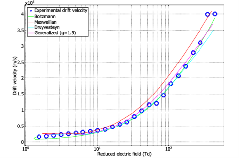
The drift velocity in the DC limit is computed from the following integral:
and in the HF limit is given by
The drift velocity is an important quantity because it provides a convenient way of comparing the results of the Boltzmann equation to experimental data.
In high frequency plasmas it is common to use the following approximation of the electron momentum equation
where νeff is an effective collision frequency and φ is a factor that is needed in order to be coherent with the drift velocity obtained from the Boltzmann equation approach here used. Substituting the HF drift velocity in the electron momentum equation it is obtained
.
In the frequency domain it is possible to derive the plasma conductivity as
.
The Townsend coefficients are computed using:
where νk is the frequency associated with the reaction rate kk. The Townsend ionization coefficient for a given gas mixture is given by
and the Townsend attachment coefficient is given by
.
When the distribution function is assumed the electric field is computed using the power balance
A plot of the drift velocity for different distribution functions versus the reduced electric field for oxygen is shown in Figure 3-1. Experimental data is also included in the plot.
Figure 3-1: Plot of experimental and computed drift velocity for different distribution functions.
The computed transport coefficients have little dependence on the type of EEDF. However, the rate coefficients for excitation and ionization processes are highly dependent on the shape of the EEDF, due to the exponential drop off in the population of electrons at energies exceeding the activation threshold. Figure 3-2 plots the ionization rate coefficient for oxygen for the types of distribution function.
Figure 3-2: Plot of ionization coefficient vs. mean electron energy for different distribution functions.