Additional Flow Resistances

Additional flow resistance due to irreversible turbulent effects in joints and junctions can be added as point conditions between pipe segments — Bends, Valves, T-junctions, Y-junctions, n-way junctions, Contractions, and Expansions. These resistances give rise to abrupt (lumped) energy losses due to turbulence in the points where they are added. The lumped pressure drop is calculated as:

(2-44)

For more information about each type, see the interface descriptions in The Pipe Flow Interface section.

Loss coefficients, Ki, for turbulent flow are available in the literature (Ref. 15) and the set predefined in the Pipe Flow interface is reproduced in the table below:

Table 2-3: Loss Coefficients
Feature	Description	Loss Coefficient K
Bends	90° standard elbow	0.9
	45° standard elbow	0.5
Valves	Globe, fully open	10
	Angle, fully open	4.4
	Gate, fully open	0.2
	Ball, fully open	4.5
	Butterfly, fully open	0.6
	Swing check, fully open	2.5
T-junction	T-junction split/merger	0.1 and 2.1 for side and main. See Figure 2-1 for a description of flow branches in a T-junction.
Contractions	Sudden
	Gradual, angle of convergence α < 22°
	Gradual, angle of convergence α > 22°
Expansions	Sudden
	Gradual, angle of convergence α < 22°
	Gradual, angle of convergence α > 22°

Above, β is the ratio of small to large cross-sectional area. The point friction losses listed above apply for Newtonian fluids. Point losses applying to non-Newtonian flow can be added as user-defined expressions, for instance from (Ref. 16).

For the point pressure loss features Bends, Valves, T-junctions, Y-junctions, n-way junctions, Contractions, and Expansions, the pressure loss can also be specified as a pressure drop Δp directly.

T-junctions

Several options to specify pressure drop across the T-junction branches are available. If the option is selected, the energy loss between main branches and junction and the energy loss between the side branch and junction are calculated as

Note that for the Nonisothermal Pipe Flow and Reacting Pipe Flow interfaces, the respective pressure drops are calculated as

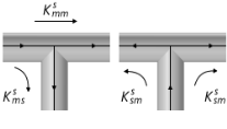
The option, which is available for the Pipe Flow interface, implements the loss coefficients according to Ref. 28. The pressure loss for a T-junction is often expressed in terms of the flow in the common branch. For joining flows, the common branch is the collector branch (Figure 2-2, left)

where

is the loss coefficient between the branch b and the common branch for joining flows.

For separating flow, the common branch is the supplier branch

For converging (joining) flow, where the collector branch is the side branch (Figure 2-2, left)

For converging flow, where the collector branch is the main branch (Figure 2-2, right)

For diverging (separating) flow, where the supplier branch is the side branch (Figure 2-3, left)

For diverging flow, where the supplier branch is the main branch (Figure 2-3, right)

The mass flow rate ratio

and the hydraulic diameters ratio

are computed automatically. Only junction with sharp corners are considered.

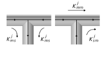
The option, that is available for the Pipe Flow interface, allows you to specify the loss coefficient in more details and account for the flow directions. Enter values or expressions for the six dimensionless loss coefficients. See Figure 2-2-Figure 2-3.

Figure 2-7: T-junction, converging flow.

Figure 2-8: T-junction, diverging flow.

The losses for the outgoing branches are calculated as

The total pressure is assume to be equal for all incoming branches:

Use the option to specify a value or expression for the pressure drop explicitly for each branch respectively:

Main 1 is the main pipe segment that has the lower index of the two in the selection list (for example, see the list in Pipe Properties).