Geometry and Mesh Settings

When particles reach the boundaries of geometric entities in a model, they do not interact with an exact parameterized representation of the geometry. Rather, they propagate through the mesh elements that discretize the modeling domain and interact with the boundary elements that cover the surfaces of the geometric entities.

When the surfaces of the geometry are flat, the shape of the surface mesh is indistinguishable from the shape of the geometric entities themselves. There is no discernible difference between the flat surfaces and their mesh representations, so it is possible to accurately compute particle trajectories even when the mesh is coarse.

Curved surfaces in the geometry, on the other hand, are susceptible to discretization error. The time and location at which the particle interacts with the boundary mesh element might be slightly different from the time at which it would have interacted with an exact representation of the surface. In addition, the tangential and normal directions on the boundary mesh element may differ from the tangential and normal directions on the surface, affecting the accuracy of boundary conditions that involve the tangential and normal directions, such as the condition which causes particles to undergo specular reflection.

The order of the curved mesh elements used to determine the geometry shape is controlled by the list in the section of the window for the main node. If , the default, is selected, the curved mesh elements are usually represented by quadratic functions.

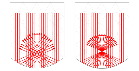
The effect of the geometry shape order is most notable on a coarse mesh, as shown in Figure 2-3. The mesh elements are shown as pale gray lines in the background and the particle trajectories are represented as thick red arrows. The particles initially move downward and are specularly reflected by a parabolic surface. If is selected from the list, all particles that hit the same boundary element are specularly reflected in the same direction, as shown on the left. Even though the bottom surface is parabolic, the particles do not all intersect at a single focus due to the discretization error. If or is selected, particles that hit the same boundary element can still be reflected in different directions because the tangential and normal directions can vary along the surface of the curved element. As a result, the particles all intersect at a well-defined focal point.

Figure 2-3: Comparison of particles being specularly reflected at a curved boundary represented using linear elements (left) and quadratic elements (right).

Particle Tracing in an Imported Mesh

It is also possible to compute particle trajectories in an imported mesh. The mesh can be imported from a COMSOL Multiphysics file (.mphbin for a binary file format or .mphtxt for a text file format) or from a NASTRAN file (.nas, .bdf, .nastran, or .dat). The particle-boundary interactions can be modeled using either linear or higher geometry shape order with the imported mesh. If is selected when importing the file, then a linear geometry shape order will be used.