Particle Tracing for Fluid Flow
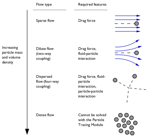
The Particle Tracing for Fluid Flow Interface is designed for modeling microscopic and macroscopic particles in a background fluid. There are two phases in the system: a particle phase consisting of discrete bubbles, particles, droplets, and so forth; and a continuous phase in which the particles are immersed. In order for the particle tracing approach to be valid, the fluid system should be a dilute or dispersed flow. This means that the volume fraction of the particles is much smaller than the volume fraction of the continuous phase, generally less than 1%. When the volume fraction of the particles is not small, the fluid system is categorized as a dense flow and a different modeling approach is required.
It is important to realize that with the particle tracing approach, particles do not displace the fluid they occupy. In addition, the finite size of the particle is not taken into account when modeling particle-wall interactions. In other words, for purposes of detecting particle-boundary interactions, the particles are treated as point masses. The specification of particle diameter is mostly used for size-dependent forces, such as the Drag Force and Dielectrophoretic Force.
Drag and Other Applied Forces
When modeling the motion of small particles in a fluid, it is important to first evaluate whether particle inertia is important enough to be included in the model. Particle inertia can be seen as a velocity lag, where larger and heavier particles change direction only gradually when the surrounding fluid changes direction, whereas smaller particles will start to match the surrounding fluid velocity almost immediately.
Particle inertia is most significant when the model particles are large and heavy, or when the surrounding fluid has very low viscosity, or a combination of the two. This is why a dust cloud might swirl around in the air before gradually settling, while a large rock quickly falls to the ground.
In the physics interface Particle Release and Propagation section, choose one of the following options from the Formulation list:
Newtonian: includes inertial terms and is therefore accurate for large particles.
Newtonian, first order: similar to Newtonian but reduces the equation order by 1 by doubling the number of dependent variables used to compute particle position.
Newtonian, ignore inertial terms: good for small particles. Assumes that the time required for a particle to accelerate in the surrounding fluid is vanishingly small.
Massless: specify the particle velocity directly. Good for tracing along streamlines.
When using the Newtonian formulation or the Newtonian, first order formulation, the maximum time step taken by the solver is determined by the smallest particles in the flow. The time-step size to fully resolve particle acceleration in the flow is proportional to the square of the particle diameter, so reducing the particle diameter by ten means that 100 times as many time steps are needed to accurately resolve the particle motion.
Sparse Flow
In a sparse flow, the continuous phase affects the motion of the particles, but the volume force exerted on the fluid by the particles is deemed insignificant. This is often referred to as a unidirectional coupling. Often the fluid velocity field can first be computed using a separate physics interface, such as the Laminar Flow interface. Then this velocity field can be used to define the drag force on the particles (via the Drag Force node). The fluid velocity can be stationary or time-dependent, whereas the particle trajectories are always computed in the time domain.
Figure 2-1: The physics features required to model sparse, dilute, and dispersed flows.
Dilute Flow
In a dilute flow the continuous phase affects the motion of the particles and the particle motion in turn disrupts the continuous phase. This is often referred to as a bidirectional coupling. The bidirectional coupling between particles and fluids can be modeled using the Fluid-Particle Interaction multiphysics coupling node. This node can be added manually if the necessary physics interfaces are already present. Alternatively, The Fluid-Particle Interaction Interface can be used to automatically add the necessary physics interfaces and multiphysics coupling nodes.
The body force exerted on the fluid by the particle is applied in an approximate way, in that it is smeared out over a mesh element. This smearing effect makes the volume force computed by the Fluid-Particle Interaction node somewhat mesh dependent. When modeling fluid-particle interactions for which the mass flow rate of particles is not constant, the continuous phase and dispersed phase must be computed simultaneously in the same study. The computational demand is significantly higher than in the Sparse Flow case.
If the fields are stationary, as often occurs when particles are released at constant mass flow rate, it may be possible to compute the particle trajectories using a Time-Dependent solver while computing the fluid flow variables using a Stationary solver. It is also possible to create a solver loop that alternates between the Stationary and Time-Dependent solvers so that a bidirectional coupling between the trajectories and fields can be established; a dedicated Bidirectionally Coupled Particle Tracing study step is available for setting up such a solver loop. The process of combining these solvers is described in the section Study Setup.
Dispersed Flow
In addition to the effects mentioned above, particle-particle interactions also need to be taken into account. This is sometimes called a “four-way coupling”. Particle-particle interactions can be included in a model by adding a Particle-Particle Interaction node.
The following limitations apply:
The Particle-Particle Interaction feature produces a Jacobian matrix that is completely full. For a large number of particles, this is very expensive to factorize. By default, the Exclude Jacobian contribution for particle-particle interaction check box is selected, which preserves the sparsity of the Jacobian. Clearing this check box is likely to result in a dramatic increase in the amount of memory and time needed to solve the problem.
Dense Flow
If the particles constitute a significant fraction of the total volume in the system, then the Particle Tracing for Fluid Flow interface cannot accurately model the particle behavior. This includes systems in which the particle diameter and the characteristic length scale of the particle’s container are similar. For example, a red blood cell in a narrow capillary would not be a valid usage case.
Computing Particle Temperature and Mass
Built-in auxiliary dependent variables for the mass and temperature can be activated by selecting the Compute particle mass and Compute particle temperature check boxes, respectively, in the Additional Variables section of the Settings window for the physics interface. When the option to compute particle mass is activated, it is possible to set the initial particle mass in particle release features, such as Release, Inlet, and Release from Grid. It is also possible to select a distribution function for the initial mass or diameter. This is important when modeling separation devices where the goal is to understand the transmission probability of particles of various sizes.
When solving for particle diameter or mass, particles may increase or decrease in size over the duration of the transient analysis. If the particles represent liquid droplets in a gas, the built-in Droplet Evaporation node can model their gradual reduction in size.
Particles can heat up or cool down due to convection and radiation. The particle temperature is treated as a constant value within each individual particle. For this to be a valid simplification, the particle Biot number must be small, meaning that heat transfer within the particle must be significantly faster than the Convective Heat Losses or Radiative Heat Losses at the surface of the particle. This limits the applicability to small particles with high thermal conductivity. Optionally, the amount of heat transferred from the particles to their surroundings can be computed and stored as a volumetric heat source or sink, using the Dissipated Particle Heat node, which could then be used as a source term when modeling a nonisothermal flow.
Particle Diffusion
The advective transport of particles due to drag and other applied forces is usually deterministic, meaning that any number of particles released from the same point and with the same initial velocity would follow the same trajectory. Sometimes particle motion also includes a diffusive component, by which particles tend to spread out over time. Two of the major phenomena that drive particle diffusion are Brownian motion and turbulent dispersion.
The Brownian Force is most significant when the particles are extremely small, generally in the submicron range. Brownian motion causes particles to drift because the number of molecules striking each particle from different sides is random, since the molecules in a fluid (even at room temperature) move around randomly and at high speeds. When the particles are larger, Brownian motion is less of a driving factor because the number of molecules hitting the particle surface is large enough that they tend to average out more readily.
Turbulent dispersion can be enabled in the settings for the Drag Force. The fluid surrounding the particles can become turbulent when its Reynolds number becomes sufficiently large. Turbulence is generally associated with faster fluid velocity, larger geometric length scale, and lower viscosity. In a turbulent flow, the fluid velocity field includes a large number of swirls or eddies that rapidly change direction.
A finite element solution that fully captures the evolution of these eddies (called direct numerical simulation or DNS) would require an inordinately high number of degrees of freedom for many practical problems; therefore the most common way to compute the fluid velocity is to solve the Reynolds-averaged Navier–Stokes (RANS) equations, which compute the average or mean-flow velocity, plus some additional transport variables that describe the average magnitude and duration of these eddies over time.
To compute particle trajectories in a turbulent flow, in the settings for the Drag Force you can select Discrete random walk or Continuous random walk from the Turbulent dispersion model list. To compute the drag force, then, the fluid velocity encountered by each particle is treated as the sum of the mean flow term and a random perturbation term.
The random perturbations due to Brownian motion and turbulent dispersion are actually pseudorandomly generated; they are not true random numbers derived from a natural entropy source. The results for different model particles will generally not be correlated with each other, but the results for the same particle may show a correlation when rerunning the study multiple times. You can manually adjust the random number seed to get new solutions, uncorrelated with the previous ones.
Particles in a Rarefied Gas
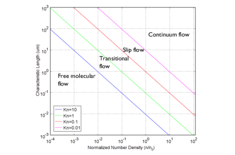
Many drag laws that are available in the Drag Force node, such as the Stokes drag law, are based on the assumption of continuum flow, in which the particle Knudsen number Kn (dimensionless) is very small,
where λ (SI unit: m) is the mean free path of molecules in the surrounding fluid, and L (SI unit: m) is a characteristic length of the particle, such as the particle diameter. The exact definition of the characteristic length may vary depending on the source being cited and should be considered with caution.
When the particles are extremely small or they are surrounded by a rarefied gas, the assumption of continuum flow may not be valid. By selecting the Include rarefaction effects check box in the physics interface Particle Release and Propagation section, it is possible to apply correction factors to the Drag Force and Thermophoretic Force, enabling accurate modeling of particle motion in the slip flow, transitional flow, and free molecular flow regimes.
Figure 2-2: A plot showing the main fluid flow regimes for rarefied gas flows. Different regimes are separated by lines of constant Knudsen numbers. The number density of the gas is normalized to the number density of an ideal gas at a pressure of 1 atmosphere and a temperature of 0°C (n0).