|
|
|
|
1
|
|
2
|
In the Select Physics tree, select Optics>Wave Optics>Electromagnetic Waves, Frequency Domain (ewfd).
|
|
3
|
Click Add.
|
|
4
|
Click
|
|
5
|
|
6
|
Click
|
|
1
|
|
2
|
|
1
|
In the Model Builder window, under Global Definitions right-click Materials and choose Blank Material.
|
|
2
|
|
1
|
|
2
|
|
1
|
|
2
|
|
1
|
|
2
|
|
3
|
|
4
|
|
1
|
|
2
|
|
3
|
|
4
|
|
1
|
In the Model Builder window, under Straight Fiber (comp1) right-click Materials and choose More Materials>Material Link.
|
|
2
|
|
1
|
|
2
|
|
3
|
|
1
|
|
2
|
|
1
|
|
2
|
|
1
|
In the Model Builder window, under Straight Fiber (comp1) right-click Definitions and choose Variables.
|
|
2
|
|
3
|
|
4
|
|
5
|
Locate the Variables section. In the table, enter the following settings:
|
|
1
|
|
2
|
|
3
|
|
1
|
|
2
|
|
3
|
|
4
|
|
5
|
|
6
|
|
7
|
|
1
|
|
2
|
|
1
|
In the Model Builder window, expand the Results>Datasets node, then click Study 1 (Straight Fiber)/Solution 1 (sol1).
|
|
2
|
|
3
|
|
1
|
|
2
|
|
3
|
|
1
|
|
2
|
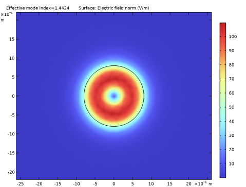
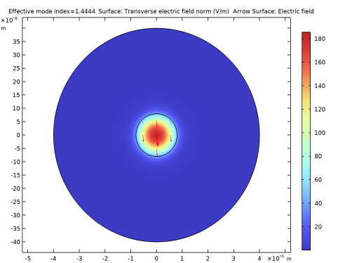
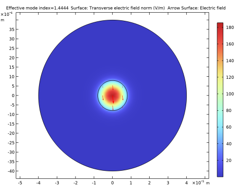
In the Settings window for Surface, click Replace Expression in the upper-right corner of the Expression section. From the menu, choose Straight Fiber (comp1)>Definitions>Variables>normEt - Transverse electric field norm - V/m. This is the variable we added in a previous step. It is clear that the plot looks almost identical to the plot of the norm of the electric field, verifying that the electric field is predominantly polarized in the transverse direction (the xy-plane).
|
|
1
|
|
2
|
In the Settings window for Arrow Surface, click Replace Expression in the upper-right corner of the Expression section. From the menu, choose Straight Fiber (comp1)>Electromagnetic Waves, Frequency Domain>Electric>ewfd.Ex,ewfd.Ey - Electric field.
|
|
3
|
In the Electric Field (ewfd) toolbar, click
 |
|
1
|
|
2
|
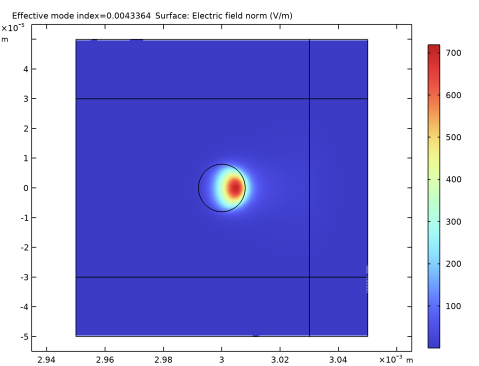
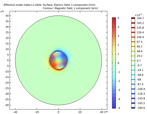
In the Settings window for Surface, click Replace Expression in the upper-right corner of the Expression section. From the menu, choose Straight Fiber (comp1)>Electromagnetic Waves, Frequency Domain>Electric>Electric field - V/m>ewfd.Ez - Electric field, z-component.
|
|
3
|
|
1
|
|
2
|
In the Settings window for Contour, click Replace Expression in the upper-right corner of the Expression section. From the menu, choose Straight Fiber (comp1)>Electromagnetic Waves, Frequency Domain>Magnetic>Magnetic field - A/m>ewfd.Hz - Magnetic field, z-component.
|
|
3
|
|
1
|
In the Model Builder window, under Results>Datasets click Study 1 (Straight Fiber)/Solution 1 (sol1).
|
|
2
|
|
1
|
|
2
|
|
1
|
|
2
|
|
3
|
|
4
|
|
1
|
|
2
|
|
3
|
|
4
|
|
5
|
|
1
|
|
2
|
|
3
|
|
4
|
|
5
|
|
6
|
|
7
|
|
1
|
|
2
|
|
3
|
|
4
|
|
5
|
|
6
|
|
1
|
|
2
|
|
3
|
|
4
|
|
5
|
|
6
|
|
7
|
|
1
|
|
2
|
|
3
|
|
4
|
|
5
|
|
1
|
Right-click Bent Fiber (comp2)>Electromagnetic Waves, Frequency Domain 2 (ewfd2) and choose Perfect Magnetic Conductor.
|
|
1
|
In the Model Builder window, under Bent Fiber (comp2) right-click Materials and choose More Materials>Material Link.
|
|
2
|
|
1
|
|
2
|
|
4
|
|
1
|
|
3
|
|
4
|
|
5
|
|
6
|
|
7
|
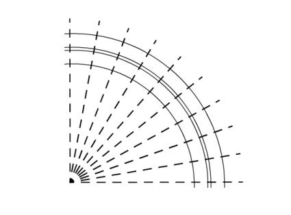
In the Typical wavelength text field, type ldaPML. This wavelength setting approximates the transverse (in the radial direction) wavelength for the mode.
|
|
1
|
|
3
|
|
4
|
|
1
|
|
2
|
|
1
|
|
2
|
|
3
|
|
4
|
|
1
|
|
2
|
|
3
|
|
1
|
|
2
|
|
3
|
|
1
|
|
2
|
|
3
|
|
1
|
|
2
|
|
3
|
|
4
|
|
1
|
|
2
|
|
3
|
Find the Studies subsection. In the Select Study tree, select Preset Studies for Selected Physics Interfaces>Mode Analysis.
|
|
4
|
Find the Physics interfaces in study subsection. In the table, clear the Solve check box for Electromagnetic Waves, Frequency Domain (ewfd).
|
|
5
|
|
6
|
|
1
|
|
2
|
|
3
|
|
4
|
|
5
|
|
6
|
|
7
|
|
1
|
In the Model Builder window, under Results>Datasets click Study 2 (Bent Fiber)/Solution 2 (3) (sol2).
|
|
2
|
|
1
|
In the Model Builder window, expand the Results>Electric Field (ewfd2) node, then click Electric Field (ewfd2).
|
|
2
|
|
3
|
|
1
|
|
2
|
|
3
|
|
4
|
|
5
|
|
6
|
Click OK.
|
|
7
|
|
8
|
|
1
|
|
2
|
|
3
|
|
4
|
|
5
|
|
6
|
|
1
|
|
2
|
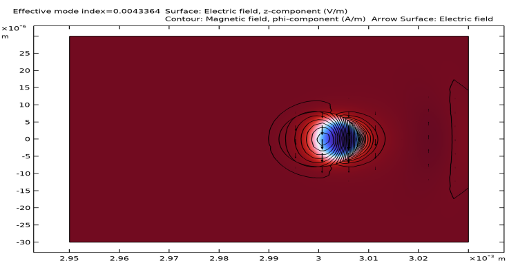
In the Settings window for Arrow Surface, click Replace Expression in the upper-right corner of the Expression section. From the menu, choose Bent Fiber (comp2)>Electromagnetic Waves, Frequency Domain 2>Electric>ewfd2.Er,ewfd2.Ez - Electric field.
|
|
3
|
|
4
|
|
1
|
|
2
|
|
3
|
|
1
|
|
2
|
|
3
|
|
1
|
|
2
|
|
1
|
|
2
|
|
3
|
|
4
|
|
5
|
|
6
|
|
7
|
|
8
|
|
1
|
|
2
|
|
3
|
|
4
|
|
5
|
|
6
|
Click Replace Expression in the upper-right corner of the Expressions section. From the menu, choose Bent Fiber (comp2)>Definitions>Variables>r0 - m.
|
|
7
|
Click
|
|
1
|
|
2
|
|
3
|
|
4
|
|
5
|
|
6
|
Locate the Expressions section. In the table, enter the following settings:
|
|
7
|
Click
|
|
1
|
|
2
|
|
3
|
|
4
|
|
5
|
|
6
|
Locate the Expressions section. In the table, enter the following settings:
|
|
7
|
Click
|
 .
.