PDF

Dielectric Slab Waveguide
Introduction
A planar dielectric slab waveguide demonstrates the principles behind any kind of dielectric waveguide such as a ridge waveguide or a step index fiber, and has a known analytic solution. This model solves for the effective index of a dielectric slab waveguide as well as for the fields, and compares to analytic results.
Figure 1: The guided modes in a dielectric slab waveguide have a known analytic solution.
Model Definition
A dielectric slab of thickness hslab = 1 μm and refractive index ncore = 1.5 forms the core of the waveguide, and sits in free space with ncladding =  1. Light polarized out of the plane of propagation, of wavelength λ =  1550 nm, is perfectly guided along the axis of the waveguide structure, as shown in Figure 1. Here, only the TE0 mode can propagate. The structure varies only in the y direction, and it is infinite and invariant in the other two directions.
The analytic solution is found by assuming that the electric field along the direction of propagation varies as Ez = E(y)exp(-ikxx), where E(y) = C1cos(kyy) inside the dielectric slab, and E(y) = C0exp(−α(|y| − (hslab/2)) in the cladding. Because the electric and magnetic fields must be continuous at the interface, the guidance condition is
where ky and α satisfy
with kcore = 2πncore and kcladding = 2πncladding. It is possible to find the solution to the above two equations via the Newton–Raphson method, which is used whenever COMSOL Multiphysics detects a system of nonlinear equations, the only requirement being that of an adequate initial guess.
This model considers a section of a dielectric slab waveguide that is finite in the x and y directions. Because the fields drop off exponentially outside the waveguide, the fields can be assumed to be zero at some distance away. This is convenient as it makes the boundary conditions in the y direction irrelevant, assuming that they are imposed sufficiently far away.
Use Numeric Port boundary conditions in the x direction to model the guided wave propagating in the positive x direction. These boundary conditions require first solving an eigenvalue problem that solves for the fields and propagation constants at the boundaries.
Results and Discussion
Figure 2 shows the results. The numeric port boundary condition at the left side excites a mode that propagates in the x direction and is perfectly absorbed by the numeric port on the right side. The analytic and numerically computed propagation constants agree.
Figure 2: The electric field in a dielectric slab waveguide.
Application Library path: Wave_Optics_Module/Verification_Examples/dielectric_slab_waveguide
Modeling Instructions
From the File menu, choose New.
New
In the New window, click  Model Wizard.
Model Wizard
1
In the Model Wizard window, click  2D.
2
In the Select Physics tree, select Optics>Wave Optics>Electromagnetic Waves, Frequency Domain (ewfd).
3
Click Add.
4
Click  Study.
5
In the Select Study tree, select Empty Study.
6
Global Definitions
Parameters 1
1
In the Model Builder window, under Global Definitions click Parameters 1.
2
In the Settings window for Parameters, locate the Parameters section.
3
Geometry 1
1
In the Model Builder window, under Component 1 (comp1) click Geometry 1.
2
In the Settings window for Geometry, locate the Units section.
3
From the Length unit list, choose µm.
Rectangle 1 (r1)
1
In the Geometry toolbar, click  Rectangle.
2
In the Settings window for Rectangle, locate the Size and Shape section.
3
In the Width text field, type w_slab.
4
In the Height text field, type h_core.
5
Locate the Position section. From the Base list, choose Center.
6
Click  Build Selected.
Rectangle 2 (r2)
1
In the Geometry toolbar, click  Rectangle.
2
In the Settings window for Rectangle, locate the Size and Shape section.
3
In the Width text field, type w_slab.
4
In the Height text field, type h_cladding.
5
Locate the Position section. From the Base list, choose Center.
6
Click  Build All Objects.
7
Click the  Zoom Extents button in the Graphics toolbar.
Electromagnetic Waves, Frequency Domain (ewfd)
Only solve for the out-of-plane electric field component, since we are only interested in solving for a transverse electric (TE) mode.
1
In the Model Builder window, under Component 1 (comp1) click Electromagnetic Waves, Frequency Domain (ewfd).
2
In the Settings window for Electromagnetic Waves, Frequency Domain, locate the Components section.
3
From the Electric field components solved for list, choose Out-of-plane vector.
The wave is excited at the port on the left side.
Port 1
1
In the Physics toolbar, click  Boundaries and choose Port.
2
3
In the Settings window for Port, locate the Port Properties section.
4
From the Type of port list, choose Numeric.
For the first port, wave excitation is on by default.
Now, add the exit port.
Port 2
1
In the Physics toolbar, click  Boundaries and choose Port.
2
3
In the Settings window for Port, locate the Port Properties section.
4
From the Type of port list, choose Numeric.
Materials
Cladding
1
In the Model Builder window, under Component 1 (comp1) right-click Materials and choose Blank Material.
2
In the Settings window for Material, type Cladding in the Label text field.
3
Locate the Material Contents section. In the table, enter the following settings:
By default, the first material you add applies on all domains. Add a core material.
Core
1
Right-click Materials and choose Blank Material.
2
In the Settings window for Material, type Core in the Label text field.
3
4
Locate the Material Contents section. In the table, enter the following settings:
Study 1
Boundary Mode Analysis
1
In the Study toolbar, click  Study Steps and choose Other>Boundary Mode Analysis.
2
In the Settings window for Boundary Mode Analysis, locate the Study Settings section.
3
In the Search for modes around text field, type n_core. This value should be in the vicinity of the value that you expect the fundamental mode to have.
4
In the Mode analysis frequency text field, type f0.
Boundary Mode Analysis 2
Add another boundary mode analysis, for the second port.
1
In the Study toolbar, click  Study Steps and choose Other>Boundary Mode Analysis.
2
In the Settings window for Boundary Mode Analysis, locate the Study Settings section.
3
In the Search for modes around text field, type n_core.
4
In the Port name text field, type 2.
5
In the Mode analysis frequency text field, type f0.
Frequency Domain
Finally, add the study step for the propagating wave in the waveguide.
1
In the Study toolbar, click  Study Steps and choose Frequency Domain>Frequency Domain.
2
In the Settings window for Frequency Domain, locate the Study Settings section.
3
In the Frequencies text field, type f0.
4
In the Study toolbar, click  Compute.
Results
Electric Field (ewfd)
The default plot shows the norm of the electric field. Modify the plot to shows the z component (compare with Figure 2).
Surface 1
1
In the Model Builder window, expand the Electric Field (ewfd) node, then click Surface 1.
2
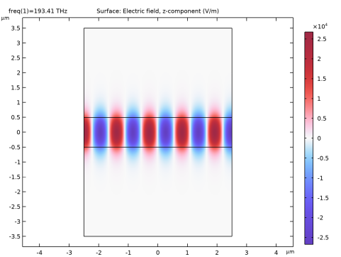
In the Settings window for Surface, click Replace Expression in the upper-right corner of the Expression section. From the menu, choose Component 1 (comp1)>Electromagnetic Waves, Frequency Domain>Electric>Electric field - V/m>ewfd.Ez - Electric field, z-component.
3
Locate the Coloring and Style section. Click  Change Color Table.
4
In the Color Table dialog box, select Wave>WaveLight in the tree.
5
6
In the Electric Field (ewfd) toolbar, click  Plot.
Now inspect the mode field plot and the effective mode index resulting from the boundary mode analysis performed for each port.
Electric Mode Field, Port 1 (ewfd)
Electric Mode Field, Port 2 (ewfd)
Finish by comparing the simulation results to the analytic solution. To compute the latter, add a Global ODEs and DAEs interface and then set up and solve the relevant equations.
Add Physics
1
In the Home toolbar, click  Add Physics to open the Add Physics window.
2
Go to the Add Physics window.
3
In the tree, select Mathematics>ODE and DAE Interfaces>Global ODEs and DAEs (ge).
4
Find the Physics interfaces in study subsection. In the table, clear the Solve check box for Study 1.
5
Click Add to Component 1 in the window toolbar.
6
In the Home toolbar, click  Add Physics to close the Add Physics window.
Add Study
1
In the Home toolbar, click  Add Study to open the Add Study window.
2
Go to the Add Study window.
3
Find the Physics interfaces in study subsection. In the table, clear the Solve check box for Electromagnetic Waves, Frequency Domain (ewfd).
4
Find the Studies subsection. In the Select Study tree, select General Studies>Stationary.
5
Click Add Study in the window toolbar.
6
In the Home toolbar, click  Add Study to close the Add Study window.
Global ODEs and DAEs (ge)
Global Equations 1
1
In the Model Builder window, under Component 1 (comp1)>Global ODEs and DAEs (ge) click Global Equations 1.
2
In the Settings window for Global Equations, locate the Global Equations section.
3
Study 2
In the Home toolbar, click  Compute.
Results
Global Evaluation 2
Finally, compare analytical and computed propagation constants.
Global Evaluation 3
1
In the Results toolbar, click  Global Evaluation.
2
In the Settings window for Global Evaluation, click Replace Expression in the upper-right corner of the Expressions section. From the menu, choose Component 1 (comp1)>Electromagnetic Waves, Frequency Domain>Ports>Propagation constants>All expressions in this group.
3
Locate the Expressions section. In the table, enter the following settings:
4
Click  Evaluate.
Global Evaluation 4
1
In the Results toolbar, click  Global Evaluation.
2
In the Settings window for Global Evaluation, locate the Data section.
3
From the Dataset list, choose Study 2/Solution 4 (sol4).
4
Locate the Expressions section. In the table, enter the following settings:
5
Click  Evaluate.