PDF

Solute Injection
Introduction
This is a benchmark case for modeling transport of contaminants through an aquifer. First a stationary Darcy flow field is computed and followed up by a transient species transport simulation. The results are compared to the benchmark situation (Ref. 1).
In addition, this model shows how to use the adaptive mesh refinement algorithm to obtain a proper mesh which resolves the given problem accurately.
Model Definition
The model geometry is depicted below.
Figure 1: Geometry for the benchmark case.
The contaminant source is located at x = y =150 m. The benchmark assumes an aquifer thickness of b = 10 m. To take this thickness in to account and compare the solutions all source terms will be scaled by this value.
Fluid Flow
Darcy’s Law is used to compute the flow field. Constant heads on the left and right hand side are applied. At the top and bottom boundary no flow condition is used. Water with density ρf is pumped at a rate W = 1 m³/d into the aquifer. A mass flux of N0 = ρf W/b is applied as point source.
Contaminant Transport
The contaminant is transported by convection, diffusion, and dispersion. The relation of longitudinal to transverse dispersivity is 10 to 3.
On the left boundary a fixed concentration = 0 is applied to reproduce the benchmark case. All other boundaries are defined as outflow boundaries. The species concentration c0 at the source is 1 kg/m3. A molar mass of M = 1 g/mol is assumed to obtain a molar concentration of 1000 mol/m3. Hence, the mass source at the point is defined according to q =c0W/(Mb).
Results and Discussion
The stationary flow field is shown in Figure 2. As expected the flow field itself is almost unaffected by the point source.
Figure 2: Stationary Darcy velocity field and hydraulic head.
Figure 3 and Figure 4 show different plots for the concentration distribution after 360 days.
Figure 3: Concentration distribution after 360 days.
Figure 4: Concentration contours after 360 days.
Notes About the COMSOL Implementation
This model makes use of the adaptive mesh refinement algorithm to get a proper mesh resolution. It is based on an error estimation such that regions with strong gradients, like the point source will be resolved with finer mesh elements than regions with small gradients.
Reference
1. C. Zheng and P. Wang, MT3DMS: A Modular Three-Dimensional Multispecies Transport Model for Simulation of Advection, Dispersion and Chemical Reactions of Contaminants in Groundwater Systems, University of Alabama, 1998.
Application Library path: Subsurface_Flow_Module/Verification_Examples/solute_injection
Modeling Instructions
From the File menu, choose New.
New
In the New window, click  Model Wizard.
Model Wizard
1
In the Model Wizard window, click  2D.
2
In the Select Physics tree, select Fluid Flow>Porous Media and Subsurface Flow>Darcy’s Law (dl).
3
Click Add.
4
In the Select Physics tree, select Chemical Species Transport>Transport of Diluted Species in Porous Media (tds).
5
Click Add.
6
Click  Study.
7
In the Select Study tree, select General Studies>Stationary.
8
Global Definitions
Parameters 1
1
In the Model Builder window, under Global Definitions click Parameters 1.
2
In the Settings window for Parameters, locate the Parameters section.
3
Geometry 1
Rectangle 1 (r1)
1
In the Geometry toolbar, click  Rectangle.
2
In the Settings window for Rectangle, locate the Size and Shape section.
3
In the Width text field, type 450.
4
In the Height text field, type 300.
Point 1 (pt1)
1
In the Geometry toolbar, click  Point.
2
In the Settings window for Point, locate the Point section.
3
In the x text field, type 150.
4
In the y text field, type 150.
5
Click  Build All Objects.
Darcy’s Law (dl)
Porous Matrix 1
1
In the Model Builder window, under Component 1 (comp1)>Darcy’s Law (dl)>Porous Medium 1 click Porous Matrix 1.
2
In the Settings window for Porous Matrix, locate the Matrix Properties section.
3
From the Permeability model list, choose Hydraulic conductivity.
4
In the K text field, type 1[m/d].
Hydraulic Head 1
1
In the Physics toolbar, click  Boundaries and choose Hydraulic Head.
2
3
In the Settings window for Hydraulic Head, locate the Hydraulic Head section.
4
In the H0 text field, type H_in.
Hydraulic Head 2
1
In the Physics toolbar, click  Boundaries and choose Hydraulic Head.
2
Line Mass Source 1
1
In the Physics toolbar, click  Points and choose Line Mass Source.
2
3
In the Settings window for Line Mass Source, locate the Line Mass Source section.
4
In the N0 text field, type W/b*rho_f.
Transport of Diluted Species in Porous Media (tds)
Use quadratic shape functions. This results in a smoother solution.
1
In the Model Builder window, under Component 1 (comp1) click Transport of Diluted Species in Porous Media (tds).
2
In the Settings window for Transport of Diluted Species in Porous Media, click to expand the Discretization section.
3
From the Concentration list, choose Quadratic.
Fluid 1
1
In the Model Builder window, under Component 1 (comp1)>Transport of Diluted Species in Porous Media (tds)>Porous Medium 1 click Fluid 1.
2
In the Settings window for Fluid, locate the Convection section.
3
From the u list, choose Darcy’s velocity field (dl/porous1).
4
Locate the Diffusion section. From the Effective diffusivity model list, choose No correction.
Porous Medium 1
In the Model Builder window, click Porous Medium 1.
Dispersion 1
1
In the Physics toolbar, click  Attributes and choose Dispersion.
2
In the Settings window for Dispersion, locate the Dispersion section.
3
Select the Specify dispersion for each species individually check box.
4
From the Dispersion tensor list, choose Dispersivity.
5
In the αL,c text field, type 10.
6
In the αT,c text field, type 3.
Concentration 1
1
In the Physics toolbar, click  Boundaries and choose Concentration.
2
3
In the Settings window for Concentration, locate the Concentration section.
4
Select the Species c check box.
Outflow 1
1
In the Physics toolbar, click  Boundaries and choose Outflow.
2
Line Mass Source 1
1
In the Physics toolbar, click  Points and choose Line Mass Source.
2
3
Type c_in*W/b.
Materials
Material 1 (mat1)
1
In the Model Builder window, under Component 1 (comp1) right-click Materials and choose Blank Material.
2
In the Settings window for Material, locate the Material Contents section.
3
Definitions
Variables 1
1
In the Model Builder window, under Component 1 (comp1) right-click Definitions and choose Variables.
2
In the Settings window for Variables, locate the Variables section.
3
Mesh 1
To build a proper mesh that resolves the strong gradients at the point use an adaptive mesh refinement algorithm. First, change the mesh resolution to finer. This is the initial mesh.
1
In the Model Builder window, under Component 1 (comp1) click Mesh 1.
2
In the Settings window for Mesh, locate the Physics-Controlled Mesh section.
3
From the Element size list, choose Finer.
Study 1
Step 1: Stationary
Calculate the stationary Darcy flow field with adaptive mesh refinement.
1
In the Model Builder window, under Study 1 click Step 1: Stationary.
2
In the Settings window for Stationary, locate the Physics and Variables Selection section.
3
In the table, clear the Solve for check box for Transport of Diluted Species in Porous Media (tds).
4
Click to expand the Adaptation and Error Estimates section. From the Adaptation and error estimates list, choose Adaptation and error estimates.
5
Clear the Save solution on every adapted mesh check box.
This saves the solution on the final mesh only.
6
Find the Mesh adaptation subsection. From the Adaptation method list, choose Rebuild mesh.
This means that a completely new mesh is built.
7
In the Home toolbar, click  Compute.
Results
Hydraulic Head
Some plots are created automatically. Create a new plot to display the hydraulic head and add an arrow plot for the velocity field as in Figure 2.
1
In the Home toolbar, click  Add Plot Group and choose 2D Plot Group.
2
In the Settings window for 2D Plot Group, type Hydraulic Head in the Label text field.
3
Locate the Data section. From the Dataset list, choose Study 1/Adaptive Mesh Refinement Solutions 1 (sol2).
Surface 1
1
Right-click Hydraulic Head and choose Surface.
2
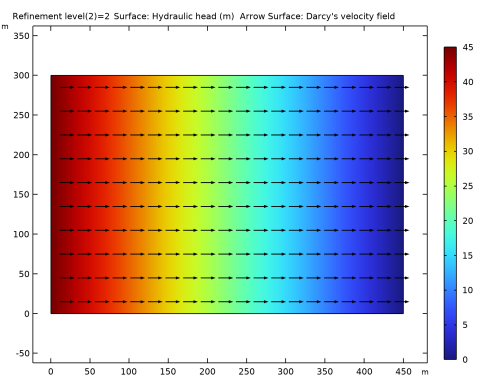
In the Settings window for Surface, click Replace Expression in the upper-right corner of the Expression section. From the menu, choose Component 1 (comp1)>Darcy’s Law>Velocity and pressure>dl.H - Hydraulic head - m.
3
In the Hydraulic Head toolbar, click  Plot.
Arrow Surface 1
1
In the Model Builder window, right-click Hydraulic Head and choose Arrow Surface.
2
In the Settings window for Arrow Surface, locate the Arrow Positioning section.
3
Find the Y grid points subsection. In the Points text field, type 10.
4
Find the X grid points subsection. In the Points text field, type 20.
5
Locate the Coloring and Style section. From the Color list, choose Black.
6
In the Hydraulic Head toolbar, click  Plot.
The velocity field is almost homogeneous. This means that the point source term does not disturb the flow field much (see Figure 2).
Component 1 (comp1)
Investigate the different mesh levels. You can find them under the Meshes node.
Level 2 Adapted Mesh 2
The Level 2 Refined Mesh 2 resolves the point source very well.
Now, run the time dependent solute transport on the finest mesh.
1
From the Home menu, choose Add Study.
Add Study
1
Go to the Add Study window.
2
Find the Studies subsection. In the Select Study tree, select General Studies>Time Dependent.
3
Find the Physics interfaces in study subsection. In the table, clear the Solve check box for Darcy’s Law (dl).
4
Click Add Study in the window toolbar.
5
From the Home menu, choose Add Study.
Study 2
Step 1: Time Dependent
1
In the Settings window for Time Dependent, locate the Study Settings section.
2
From the Time unit list, choose d.
3
In the Output times text field, type range(0,10,365).
4
Click to expand the Mesh Selection section. The refined mesh is selected automatically.
5
Click to expand the Values of Dependent Variables section. Find the Initial values of variables solved for subsection. From the Settings list, choose User controlled.
6
From the Method list, choose Solution.
7
Find the Values of variables not solved for subsection. From the Settings list, choose User controlled.
8
From the Method list, choose Solution.
9
From the Study list, choose Study 1, Stationary.
10
In the Model Builder window, expand the Component 1 (comp1)>Meshes node.
11
Right-click Study 2 and choose Compute.
Results
Create a new plot to reproduce Figure 3.
Concentration, Height Expression
1
In the Home toolbar, click  Add Plot Group and choose 2D Plot Group.
2
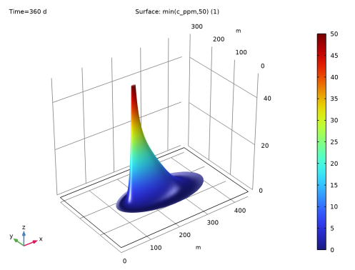
In the Settings window for 2D Plot Group, type Concentration, Height Expression in the Label text field.
3
Locate the Data section. From the Dataset list, choose Study 2/Solution 6 (sol6).
Surface 1
1
Right-click Concentration, Height Expression and choose Surface.
2
In the Settings window for Surface, locate the Expression section.
3
In the Expression text field, type min(c_ppm,50).
4
Click to expand the Range section. Select the Manual data range check box.
5
In the Minimum text field, type 0.1.
6
In the Maximum text field, type 50.
7
In the Concentration, Height Expression toolbar, click  Plot.
Height Expression 1
Right-click Surface 1 and choose Height Expression.
Create the contour plot as in Figure 4 with the following steps.
Concentration Contours
1
In the Home toolbar, click  Add Plot Group and choose 2D Plot Group.
2
In the Settings window for 2D Plot Group, type Concentration Contours in the Label text field.
3
Locate the Data section. From the Dataset list, choose Study 2/Solution 6 (sol6).
Contour 1
1
Right-click Concentration Contours and choose Contour.
2
In the Settings window for Contour, click Replace Expression in the upper-right corner of the Expression section. From the menu, choose Component 1 (comp1)>Definitions>Variables>c_ppm - Concentration (ppm).
3
Locate the Levels section. From the Entry method list, choose Levels.
4
In the Levels text field, type 0.1 1 10 50.
5
Locate the Coloring and Style section. From the Coloring list, choose Uniform.
6
From the Color list, choose Black.
7
Select the Level labels check box.
8
In the Precision text field, type 2.
9
Clear the Color legend check box.
10
In the Concentration Contours toolbar, click  Plot.