|
|
|


|
•
|
Elastic data: instantaneous shear modulus G0 = 27.46 GPa and long-term shear modulus of G = μ0G0, bulk modulus K = 39.88 GPa.
|
|
•
|
|
•
|
Thermal properties: A WLF shift function is used with C1 = 17.44 and C2 = 51.6. These values are reasonable approximations for many polymers.
|
|
•
|
The reference temperature is 500 K.
|
|
•
|
|
•
|
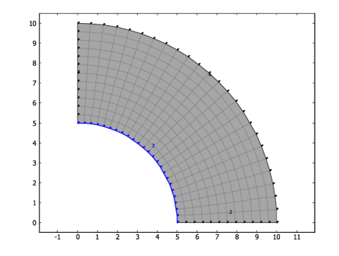
Stationary analysis: The inner and outer circular edges both have a temperature distribution varying linearly with the y-coordinate from 500 K at the y = 0 symmetry section to 506 K at the x = 0 symmetry section.
|
|
1
|
|
2
|
|
3
|
Click Add.
|
|
4
|
|
5
|
Click Add.
|
|
6
|
Click
|
|
1
|
|
2
|
|
1
|
|
2
|
|
3
|
|
1
|
|
2
|
|
3
|
|
4
|
|
5
|
Click to expand the Layers section. In the table, enter the following settings:
|
|
1
|
|
2
|
|
3
|
|
4
|
On the object c1, select Domain 1 only.
|
|
5
|
|
1
|
|
2
|
|
3
|
From the list, choose Quasistatic.
|
|
1
|
In the Model Builder window, under Component 1 (comp1)>Solid Mechanics (solid) click Linear Elastic Material 1.
|
|
2
|
|
3
|
|
1
|
|
2
|
|
4
|
Click
|
|
6
|
Click
|
|
8
|
Click
|
|
10
|
|
11
|
|
12
|
Locate the Viscoelasticity Model section. From the Stiffness used in stationary studies list, choose Instantaneous.
|
|
1
|
|
1
|
|
3
|
|
4
|
|
5
|
|
6
|
|
1
|
|
3
|
|
4
|
|
1
|
In the Model Builder window, under Component 1 (comp1) right-click Materials and choose Blank Material.
|
|
3
|
|
1
|
|
3
|
|
4
|
|
1
|
|
3
|
|
4
|
|
5
|
|
1
|
|
2
|
|
3
|
|
4
|
|
5
|
|
1
|
|
2
|
|
3
|
|
1
|
|
2
|
|
1
|
In the Model Builder window, under Results, Ctrl-click to select Stress (solid), Temperature (ht), and Isothermal Contours (ht).
|
|
2
|
Right-click and choose Group.
|
|
1
|
|
2
|
|
3
|
|
4
|
|
5
|
|
1
|
|
2
|
In the Settings window for Study, type Study: Transient (Constant Temperature) in the Label text field.
|
|
1
|
In the Model Builder window, under Study: Transient (Constant Temperature) click Step 1: Time Dependent.
|
|
2
|
|
3
|
In the Output times text field, type range(0,20,200) range(250,50,1000) range(1100,100,2000) range(2200,200,7200).
|
|
1
|
|
2
|
|
3
|
|
4
|
|
5
|
|
6
|
|
7
|
|
8
|
In the Model Builder window, under Study: Transient (Constant Temperature)>Solver Configurations>Solution 2 (sol2) click Time-Dependent Solver 1.
|
|
9
|
|
10
|
|
11
|
|
1
|
|
2
|
|
3
|
|
4
|
|
5
|
Locate the Data section. From the Dataset list, choose Study: Transient (Constant Temperature)/Solution 2 (sol2).
|
|
1
|
|
2
|
|
3
|
|
4
|
|
5
|
Locate the Data section. From the Dataset list, choose Study: Transient (Constant Temperature)/Solution 2 (sol2).
|
|
1
|
|
2
|
|
3
|
|
4
|
|
5
|
|
6
|
|
7
|
|
8
|
|
1
|
|
2
|
|
3
|
|
4
|
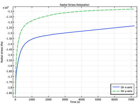
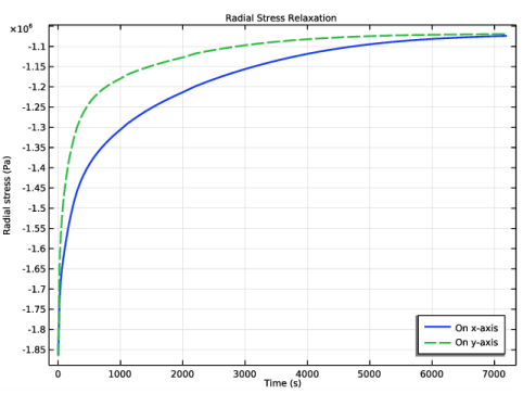
Click Replace Expression in the upper-right corner of the y-Axis Data section. From the menu, choose Component 1 (comp1)>Solid Mechanics>Stress>Stress tensor (spatial frame) - N/m²>solid.sxx - Stress tensor, xx-component.
|
|
5
|
|
6
|
|
7
|
|
1
|
In the Model Builder window, right-click Stress Relaxation (Constant Temperature) and choose Point Graph.
|
|
2
|
|
3
|
|
4
|
Click Replace Expression in the upper-right corner of the y-Axis Data section. From the menu, choose Component 1 (comp1)>Solid Mechanics>Stress>Stress tensor (spatial frame) - N/m²>solid.syy - Stress tensor, yy-component.
|
|
5
|
|
6
|
|
7
|
|
8
|
|
1
|
|
2
|
|
3
|
|
1
|
In the Model Builder window, under Results, Ctrl-click to select Stress (solid) 1, Temperature (ht) 1, Isothermal Contours (ht) 1, and Stress Relaxation (Constant Temperature).
|
|
2
|
Right-click and choose Group.
|
|
1
|
|
2
|
|
3
|
|
4
|
|
5
|
|
1
|
|
2
|
In the Output times text field, type range(0,20,200) range(250,50,1000) range(1100,100,2000) range(2200,200,7200).
|
|
3
|
Locate the Physics and Variables Selection section. Select the Modify model configuration for study step check box.
|
|
4
|
|
5
|
Right-click and choose Disable.
|
|
6
|
|
7
|
In the Settings window for Study, type Study: Transient (Variable Temperature) in the Label text field.
|
|
1
|
|
2
|
|
3
|
|
4
|
|
5
|
|
6
|
|
7
|
|
8
|
In the Model Builder window, under Study: Transient (Variable Temperature)>Solver Configurations>Solution 3 (sol3) click Time-Dependent Solver 1.
|
|
9
|
|
10
|
|
11
|
|
1
|
In the Model Builder window, under Results>Datasets right-click Cut Point 2D 1 and choose Duplicate.
|
|
2
|
|
3
|
|
1
|
In the Model Builder window, under Results>Datasets right-click Cut Point 2D 2 and choose Duplicate.
|
|
2
|
|
3
|
|
1
|
In the Model Builder window, right-click Stress Relaxation (Constant Temperature) and choose Duplicate.
|
|
2
|
|
3
|
|
4
|
|
5
|
In the Settings window for 1D Plot Group, type Stress Relaxation (Variable Temperature) in the Label text field.
|
|
1
|
In the Model Builder window, expand the Stress Relaxation (Variable Temperature) node, then click Point Graph 1.
|
|
2
|
|
3
|
|
1
|
|
2
|
|
3
|
|
4
|
|
1
|
In the Model Builder window, under Results, Ctrl-click to select Stress (solid) 2, Temperature (ht) 2, Isothermal Contours (ht) 2, and Stress Relaxation (Variable Temperature).
|
|
2
|
Right-click and choose Group.
|