PDF

Buckling Analysis of a Truss Tower
Introduction
Trusses are commonly used to create light structures that can support heavy loads. When designing such a structure, it is important to ensure its safety. For a tower made of bars, buckling can cause the structure to collapse. This example shows how to compute the critical buckling load using a linear buckling analysis. The solution is compared with an analytical expression for critical load estimation for Euler buckling.
Then a slight prescribed deformation is applied to the structure, and a stationary study with load increasing up to critical buckling load is performed. This study puts in evidence the singularity at critical buckling load.
Model Definition
The model geometry consists of a 19 m tall truss tower with a rectangular section. The critical buckling load is computed using the linear buckling analysis available in the Truss interface.
The geometry is the periodic structure represented in Figure 1 below. It consists of 19 blocks of trusses. Each block has a width of 0.45 m, a depth of 0.40 m and a height of 1.0 m. The trusses that are perpendicular to the ground are thicker and have an outer radius of 15 mm and an inner radius of 10 mm. The remaining trusses have an outer radius of 10 mm and an inner radius of 7 mm. The tower is made out of structural steel, which is one of the predefined materials in the material library.
Figure 1: Geometry of the truss tower.
The tower is fixed at the ground level and a vertical load is applied at the top.
One fourth of the unit load is applied at each point of the tower top so that the critical load factor returned by the linear buckling analysis corresponds to the load that would cause the collapse of the structure.
A second study is performed to put in evidence the singularity at critical buckling load. To do so, the geometry is slightly deformed according to the first mode shape to initiate the buckling deformation. The load is then increased above the calculated critical buckling load in a stationary study using an auxiliary sweep.
Results and Discussion
For a simple column the critical buckling load is given by the Euler buckling formula
where E is the Young’s modulus, I is the area moment of inertia, L is the unsupported length of the column and K is the column effective length factor.
For a column with one end fixed and the other end free to move laterally, K = 2.
For a tower like the one in this example with 4 main bars in the axial direction, the area of moment of inertia of the section can be computed as:
where h is the distance between the vertical bars, and S the cross section area of the bars.
As the section is rectangular with different depth and width values, the tower has one weak direction. Here the depth is 40 cm and the width is 45 cm. This means that the first critical buckling load is expected to be about 86 kN in the depth direction (y direction). In the width direction, which is expected to be stiffer, the critical buckling load is estimated to be about 110 kN.
The results obtained with the linear buckling analysis agree well with these values. Note that the approximation given for the Euler buckling critical load is suitable for a tower structure when the height is significantly larger than the width or the depth.
Figure 2 shows the value of the first critical buckling load and the deformation shape.
Figure 2: Deformation shape at the first critical buckling load.
Figure 3 shows the value of the second critical buckling load and the deformation shape.
Figure 3: Deformation shape at the second critical buckling load.
In addition to the buckling of the whole structure, the safety against buckling of individual truss members must be studied. The critical compressive load for an individual bar can be calculated from material properties and the geometry of the bar:
Here, Imin is the moment of inertia in the weakest direction, based on the cross section data, and Lbar is the length of the bar. In this case the effective length factor Kbar is kept to its default value of 1, which corresponds to a pinned-pinned configuration. From this critical force and the compressive axial force N, the failure index fi and the local buckling safety factor sf can be calculated:
Based on the stationary step with unit loading it appears that the maximum buckling failure index is reached for some diagonal bars near the top of the tower (Figure 4), which undergo less compressive force than vertical bars, but are longer and thinner. The calculated minimal value of safety factor leads to a critical load of about 150 kN, which is significantly higher than the critical load of the two first modes for global buckling. Hence the global buckling will occur before the collapse of the individual truss members.
Figure 4: Maximum local buckling index, with value of minimal safety factor.
The plot of the force in post buckling analysis (Figure 5) shows that the higher forces are located at the base of the tower, while the points at the top of the tower have the maximum horizontal displacement. The displacement plot shows a sudden increase around the critical load, see Figure 6. The stress plot (Figure 7) also shows a sudden increase of the stress at critical load. The stress value becomes very high, probably higher than the physical limits of the material, which may cause a total collapse of the structure.
Figure 5: Force in truss at critical load.
Figure 6: Displacement of the top of the tower in post buckling study.
Figure 7: Stress in the truss at critical load.
Notes About the COMSOL Implementation
The settings of the post buckling analysis are made easier by the Buckling Imperfection node.
It contains a Deformed Geometry section that enables to choose the buckling solution and modes that will defined the prescribed displacements. The Create button generates one Prescribed Deformation node for each structural mechanics physics interface involved, and sets the prescribed deformations with the variables defined by the node. The prescribed deformations are those computed in the linear buckling study, multiplied by the scale factor. Low values of scale factor make the buckling effect sharper, but lead to more difficult convergence.
The Nonlinear Buckling Study section enables to select an existing study or choose to create a new one, and choose a parameter used to increase the loads in an auxiliary sweep. The Create button then creates a new stationary study if required, then checks Include geometric nonlinearities on, and applies an auxiliary sweep with the selected parameter. The parameters values are filled based on the calculated critical buckling factor, with a logarithmic increase to capture accurately the behavior near the singularity.
Application Library path: Structural_Mechanics_Module/Buckling_and_Wrinkling/truss_tower_buckling
Modeling Instructions
From the File menu, choose New.
New
In the New window, click  Model Wizard.
Model Wizard
1
In the Model Wizard window, click  3D.
2
In the Select Physics tree, select Structural Mechanics>Truss (truss).
3
Click Add.
4
Click  Study.
5
In the Select Study tree, select Preset Studies for Selected Physics Interfaces>Linear Buckling.
6
Global Definitions
Geometric Parameters
1
In the Model Builder window, under Global Definitions click Parameters 1.
2
In the Settings window for Parameters, type Geometric Parameters in the Label text field.
3
Locate the Parameters section. Click  Load from File.
4
Loads
1
In the Home toolbar, click  Parameters and choose Add>Parameters.
2
In the Settings window for Parameters, type Loads in the Label text field.
3
Locate the Parameters section. In the table, enter the following settings:
Geometry 1
Block 1 (blk1)
1
In the Geometry toolbar, click  Block.
2
In the Settings window for Block, locate the Size and Shape section.
3
In the Width text field, type width.
4
In the Depth text field, type depth.
5
In the Height text field, type height.
Polygon 1 (pol1)
1
In the Geometry toolbar, click  More Primitives and choose Polygon.
2
In the Settings window for Polygon, locate the Object Type section.
3
From the Type list, choose Closed curve.
4
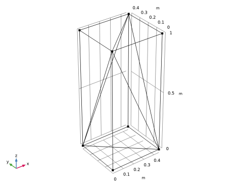
Locate the Coordinates section. In the table, enter the following settings:
Line Segment 1 (ls1)
1
In the Geometry toolbar, click  More Primitives and choose Line Segment.
2
In the Settings window for Line Segment, locate the Starting Point section.
3
From the Specify list, choose Coordinates.
4
Locate the Endpoint section. From the Specify list, choose Coordinates.
5
Locate the Starting Point section. In the y text field, type depth.
6
Locate the Endpoint section. In the x text field, type width.
Line Segment 2 (ls2)
1
In the Geometry toolbar, click  More Primitives and choose Line Segment.
2
In the Settings window for Line Segment, locate the Starting Point section.
3
From the Specify list, choose Coordinates.
4
Locate the Endpoint section. From the Specify list, choose Coordinates.
5
Locate the Starting Point section. In the z text field, type height.
6
Locate the Endpoint section. In the x text field, type width, y to depth, and z to height.
Convert to Curve 1 (ccur1)
1
In the Geometry toolbar, click  Conversions and choose Convert to Curve.
2
Click in the Graphics window and then press Ctrl+A to select all objects.
3
In the Geometry toolbar, click  Build All.
Mirror 1 (mir1)
1
In the Geometry toolbar, click  Transforms and choose Mirror.
2
3
In the Settings window for Mirror, locate the Input section.
4
Select the Keep input objects check box.
5
Locate the Point on Plane of Reflection section. In the z text field, type height.
6
In the Geometry toolbar, click  Build All.
Array 1 (arr1)
1
In the Geometry toolbar, click  Transforms and choose Array.
2
3
In the Settings window for Array, locate the Size section.
4
In the z size text field, type n.
5
Locate the Displacement section. In the z text field, type 2*height.
Array 2 (arr2)
1
In the Geometry toolbar, click  Transforms and choose Array.
2
3
In the Settings window for Array, locate the Size section.
4
In the z size text field, type n-1.
5
Locate the Displacement section. In the z text field, type 2*height.
6
In the Geometry toolbar, click  Build All.
7
Click the  Go to Default View button in the Graphics toolbar.
Create selections for vertical and transversal edges to make further modeling easier.
Definitions
Vertical Edges
1
In the Definitions toolbar, click  Explicit.
2
In the Settings window for Explicit, type Vertical Edges in the Label text field.
3
Locate the Input Entities section. From the Geometric entity level list, choose Edge.
4
5
Select the Group by continuous tangent check box.
Transversal Edges
1
In the Definitions toolbar, click  Complement.
2
In the Settings window for Complement, type Transversal Edges in the Label text field.
3
Locate the Geometric Entity Level section. From the Level list, choose Edge.
4
Locate the Input Entities section. Under Selections to invert, click  Add.
5
In the Add dialog box, select Vertical Edges in the Selections to invert list.
6
Add Material
1
In the Home toolbar, click  Add Material to open the Add Material window.
2
Go to the Add Material window.
3
In the tree, select Built-in>Structural steel.
4
Click Add to Component in the window toolbar.
5
In the Home toolbar, click  Add Material to close the Add Material window.
Truss (truss)
Cross-Section Data 1
1
In the Model Builder window, under Component 1 (comp1)>Truss (truss) click Cross-Section Data 1.
2
In the Settings window for Cross-Section Data, locate the Cross-Section Definition section.
3
From the list, choose Common sections.
4
From the Section type list, choose Pipe.
5
In the do text field, type do1.
6
In the di text field, type di1.
Cross-Section Data 2
1
In the Physics toolbar, click  Edges and choose Cross-Section Data.
2
In the Settings window for Cross-Section Data, locate the Edge Selection section.
3
From the Selection list, choose Transversal Edges.
4
Locate the Cross-Section Definition section. From the list, choose Common sections.
5
From the Section type list, choose Pipe.
6
In the do text field, type do2.
7
In the di text field, type di2.
Pinned 1
1
In the Physics toolbar, click  Points and choose Pinned.
2
In the Settings window for Pinned, locate the Point Selection section.
3
Click  Paste Selection.
4
In the Paste Selection dialog box, type 1 21 41 61 in the Selection text field.
5
Point Load 1
1
In the Physics toolbar, click  Points and choose Point Load.
2
In the Settings window for Point Load, locate the Point Selection section.
3
Click  Paste Selection.
4
In the Paste Selection dialog box, type 20 40 60 80 in the Selection text field.
5
6
In the Settings window for Point Load, locate the Force section.
7
Specify the FP vector as
Study 1
Step 2: Linear Buckling
1
In the Model Builder window, under Study 1 click Step 2: Linear Buckling.
2
In the Settings window for Linear Buckling, locate the Study Settings section.
3
In the Desired number of buckling modes text field, type 2.
4
In the Home toolbar, click  Compute.
Results
Line 1
1
In the Model Builder window, expand the Mode Shape (truss) node, then click Line 1.
2
In the Settings window for Line, click to expand the Title section.
3
From the Title type list, choose None.
4
Locate the Coloring and Style section. In the Radius scale factor text field, type 4.
5
Click the  Show Grid button in the Graphics toolbar.
6
In the Mode Shape (truss) toolbar, click  Plot.
Create a new plot to check that local buckling of truss members occurs at higher load than the global buckling.
Local Buckling
1
In the Home toolbar, click  Add Plot Group and choose 3D Plot Group.
2
In the Settings window for 3D Plot Group, type Local Buckling in the Label text field.
3
Locate the Data section. From the Dataset list, choose Study 1/Solution Store 1 (sol2).
Line 1
1
Right-click Local Buckling and choose Line.
2
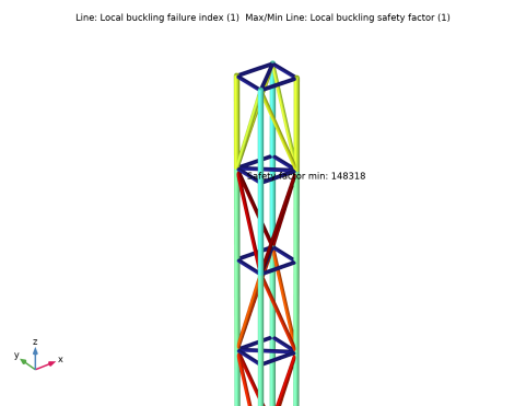
In the Settings window for Line, click Replace Expression in the upper-right corner of the Expression section. From the menu, choose Component 1 (comp1)>Truss>Safety>Local buckling>truss.lbf_i - Local buckling failure index.
3
Locate the Coloring and Style section. Clear the Color legend check box.
4
Click to expand the Quality section. From the Smoothing list, choose None.
5
Locate the Coloring and Style section. From the Line type list, choose Tube.
6
In the Tube radius expression text field, type truss.re.
7
Select the Radius scale factor check box. In the associated text field, type 2.
Local Buckling
In the Model Builder window, click Local Buckling.
Max/Min Line 1
1
In the Local Buckling toolbar, click  More Plots and choose Max/Min Line.
2
In the Settings window for Max/Min Line, click Replace Expression in the upper-right corner of the Expression section. From the menu, choose Component 1 (comp1)>Truss>Safety>Local buckling>truss.lbs_f - Local buckling safety factor.
3
Locate the Display section. From the Display list, choose Min.
4
Locate the Text Format section. In the Prefix text field, type Safety factor .
5
In the Local Buckling toolbar, click  Plot.
Now prescribe a deformation to the geometry from the calculated buckling mode to perform a post-buckling study.
Definitions
Buckling Imperfection 1 (bcki1)
1
In the Definitions toolbar, click  Physics Utilities and choose Buckling Imperfection.
2
In the Settings window for Buckling Imperfection, locate the Deformed Geometry section.
3
Find the Mode selection subsection. In the table, enter the following settings:
4
Click Configure in the upper-right corner of the Deformed Geometry section.
This button creates a Prescribed Deformation node with the requested deformation settings. The newly created Prescribed Deformation is automatically disabled in the existing study steps to enable further computation without changes in the results.
5
Locate the Nonlinear Buckling Study section. From the Load parameter list, choose load (Applied load).
6
Click Configure in the upper-right corner of the Nonlinear Buckling Study section.
This button creates a new study with stationary step, activates geometric nonlinearities and applies an auxiliary sweep for the post-buckling study.
Study 2
Solution 3 (sol3)
1
In the Model Builder window, expand the Component 1 (comp1)>Deformed Geometry node.
2
Right-click Study 2 and choose Show Default Solver.
3
In the Model Builder window, expand the Solution 3 (sol3) node.
4
In the Model Builder window, expand the Study 2>Solver Configurations>Solution 3 (sol3)>Stationary Solver 1 node, then click Fully Coupled 1.
5
In the Settings window for Fully Coupled, click to expand the Method and Termination section.
6
From the Nonlinear method list, choose Constant (Newton).
7
In the Study toolbar, click  Compute.
Results
Stress (truss)
1
In the Settings window for 3D Plot Group, locate the Data section.
2
From the Parameter value (load (N)) list, choose 84820.
Line 1
1
In the Model Builder window, expand the Stress (truss) node, then click Line 1.
2
In the Settings window for Line, locate the Expression section.
3
From the Unit list, choose MPa.
4
Locate the Coloring and Style section. In the Radius scale factor text field, type 4.
5
In the Stress (truss) toolbar, click  Plot.
6
In the Home toolbar, click  Add Predefined Plot.
Add Predefined Plot
1
Go to the Add Predefined Plot window.
2
In the tree, select Study 2/Solution 3 (sol3)>Truss>Force (Truss).
3
Click Add Plot in the window toolbar.
Results
Force (truss)
1
In the Settings window for 3D Plot Group, locate the Data section.
2
From the Parameter value (load (N)) list, choose 84820.
Line 1
1
In the Model Builder window, expand the Force (truss) node, then click Line 1.
2
In the Settings window for Line, locate the Coloring and Style section.
3
In the Radius scale factor text field, type 4.
4
In the Force (truss) toolbar, click  Plot.
Create a new plot to show the displacement with respect to applied load.
Post Buckling Displacement
1
In the Home toolbar, click  Add Plot Group and choose 1D Plot Group.
2
In the Settings window for 1D Plot Group, locate the Data section.
3
From the Dataset list, choose Study 2/Solution 3 (sol3).
4
In the Label text field, type Post Buckling Displacement.
Point Graph 1
1
Right-click Post Buckling Displacement and choose Point Graph.
2
3
In the Settings window for Point Graph, locate the y-Axis Data section.
4
In the Expression text field, type v.
5
Click to expand the Coloring and Style section. Find the Line markers subsection. From the Marker list, choose Point.
6
In the Post Buckling Displacement toolbar, click  Plot.
Post Buckling Stress
1
In the Model Builder window, right-click Post Buckling Displacement and choose Duplicate.
2
In the Settings window for 1D Plot Group, type Post Buckling Stress in the Label text field.
Point Graph 1
1
In the Model Builder window, expand the Post Buckling Stress node, then click Point Graph 1.
2
In the Settings window for Point Graph, locate the Selection section.
3
Click  Clear Selection.
4
5
Click Replace Expression in the upper-right corner of the y-Axis Data section. From the menu, choose Component 1 (comp1)>Truss>Stress>truss.mises - von Mises stress - N/m².
6
Locate the y-Axis Data section. From the Unit list, choose MPa.
7
In the Post Buckling Stress toolbar, click  Plot.