|
|
|
|
•
|
|
•
|
|
•
|
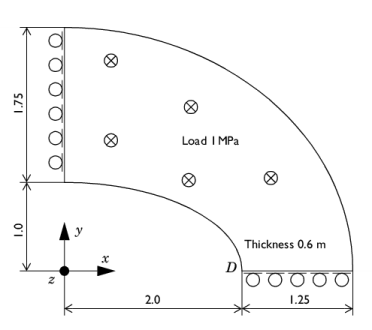
Midplane on outer ellipse surface constrained in the z direction.
|
|
1
|
|
2
|
|
3
|
Click Add.
|
|
4
|
Click
|
|
5
|
|
6
|
Click
|
|
1
|
|
2
|
|
1
|
|
2
|
|
3
|
|
4
|
|
5
|
|
6
|
|
7
|
|
1
|
|
2
|
|
3
|
|
4
|
|
5
|
|
1
|
|
2
|
|
3
|
|
4
|
|
5
|
|
6
|
|
1
|
|
2
|
|
3
|
|
4
|
|
5
|
Select the object e2 only.
|
|
6
|
|
1
|
|
2
|
|
3
|
|
4
|
Locate the Coordinates section. In the table, enter the following settings:
|
|
1
|
|
2
|
|
3
|
|
4
|
Locate the Coordinates section. In the table, enter the following settings:
|
|
5
|
|
1
|
|
2
|
Select the object dif1 only.
|
|
3
|
|
4
|
|
5
|
|
6
|
|
1
|
In the Model Builder window, under Component 1 (comp1)>Geometry 1 right-click Work Plane 1 (wp1) and choose Extrude.
|
|
2
|
|
4
|
|
5
|
|
1
|
In the Model Builder window, under Component 1 (comp1) right-click Materials and choose Blank Material.
|
|
2
|
|
1
|
In the Model Builder window, under Component 1 (comp1) right-click Solid Mechanics (solid) and choose More Constraints>Symmetry.
|
|
1
|
|
3
|
|
4
|
|
5
|
|
1
|
|
3
|
|
4
|
|
1
|
|
3
|
|
4
|
|
1
|
|
2
|
|
3
|
|
4
|
|
5
|
|
1
|
|
2
|
|
1
|
|
3
|
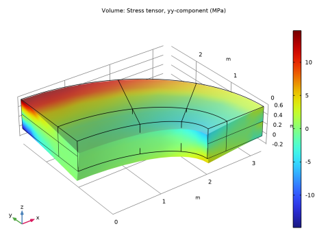
In the Settings window for Point Evaluation, click Replace Expression in the upper-right corner of the Expressions section. From the menu, choose Component 1 (comp1)>Solid Mechanics>Stress>Stress tensor (spatial frame) - N/m²>solid.syy - Stress tensor, yy-component.
|
|
4
|
Locate the Expressions section. In the table, enter the following settings:
|
|
5
|
Click
|
|
1
|
|
2
|
In the Settings window for Volume, click Replace Expression in the upper-right corner of the Expression section. From the menu, choose Component 1 (comp1)>Solid Mechanics>Stress>Stress tensor (spatial frame) - N/m²>solid.syy - Stress tensor, yy-component.
|
|
3
|
|
4
|
|
5
|
|
6
|
Click OK.
|
|
7
|