Connecting Shells and Solids

The Shell interface can be used to model thin structures in 3D. The thickness of a shell is taken into account mathematically, but is not explicitly modeled in the geometry. This makes the use of the Shell interface efficient because only boundaries have to be meshed. The Shell interface provides good results as long as the structures are thin. In practice, it sometimes happens that this requirement is not met in the entire geometry, so that local regions require a full solid model. In such a case, the Shell interface can be used for thinner parts, and then be coupled to a Solid Mechanics interface for other parts.

This example demonstrates how you model a transition from a shell to a solid. The assumptions and accuracy of such a transition is also discussed.

Model Definition

The model geometry (Figure 1) consists of a cylindrical steel pipe with three circular cutouts along its length on one side. The wall thickness of 0.1 m is small compared to the radius of 1 m. The entire structure could thus be modeled with the Shell interface. To demonstrate the connection between shells and a solid domain, the geometry is instead separated in three sections. The middle section is modeled as a solid domain that is connected to a shell on either side.

Figure 1: The geometry divided into regions modeled using shells and solids.

The model is set up with a Shell interface for the outer parts, and a Solid Mechanics interface for the solid domain in the middle. Where the edges of the shell midsurfaces meet the solid boundaries, special connection boundary conditions are added through the multiphysics coupling. Different types of conditions are used for the connection on the left and right sides, in order to highlight their properties.

The shell deformation is described with 6 DOFs, three displacement components and three components for the rotation of the shell normal. In the Solid Mechanics domain the latter DOFs are not present, as the 3D state of deformation is resolved explicitly with a 3D mesh. The 6 DOFs per node of the shell edge thus have to be connected to the 3 DOFs per node on the boundary of the connection. There are two options for this connection, and . The first type violates the shell assumptions somewhat and leads to unphysical stress states locally at the connection. This aberration disappears within a few elements from the connection and the results can be acceptable in many situations. The flexible connection introduces new solution variables, the softening functions. The benefit is more accurate stress results at the connection, but it comes with an extra computational cost. The flexible connection cannot be used if the mesh in the thickness direction of the solid is too coarse. The required number of elements needed depends on the shape function order, but with standard quadratic shape function, at least three elements are needed in the thickness direction.

Additional details about the connection types can be found in the documentation for the Shell interface. In this model, both connection types are used, one on either side of the solid domain.

Three different load cases are analyzed, so that the behavior of the two connection types can be compared for different stress states. One end of the geometry is constrained, while the other is subject to different edge loads corresponding to a tension, and torsion. A third load case is also considered where the pipe is subject to an internal pressure.

Results and Discussion

The von Mises stress distribution for the pressure load case is shown in Figure 2. The overall stress state in the shells is consistent with the results obtained in the solid domain. There is however a slight difference, since the solid captures the variation of the stress through the thickness correctly.

Figure 2: The von Mises stress distribution of the pressure load case.

The stress distribution along the top of the pipe for all three load cases is shown in Figure 3, Figure 4, and Figure 5. A closer look reveals some differences in the stress results, especially near the connected region. To interpret the graphs, note the following:

•

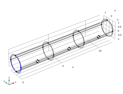
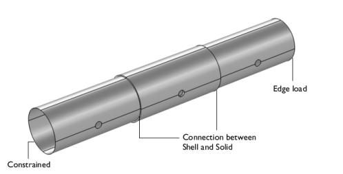
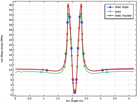
The direction of the graphs runs from the constrained end of the pipe toward the loaded end.

•

The graphs follow the perimeter of the holes.

•

The left end of the Shell, Rigid graph is at the constrained end. The constraint may cause local disturbances there.

•

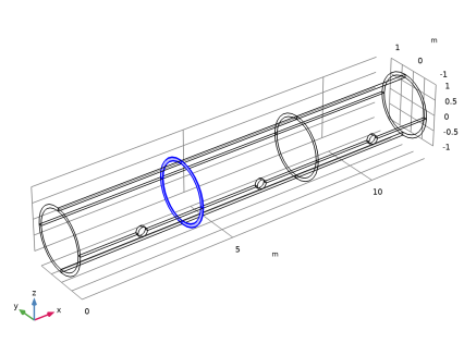
The right end of the Shell, Rigid graph is connected to the left end of the Solid graph at the rigid connection.

•

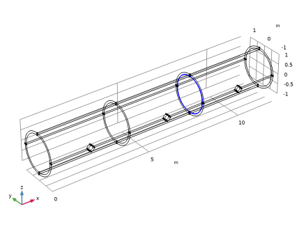
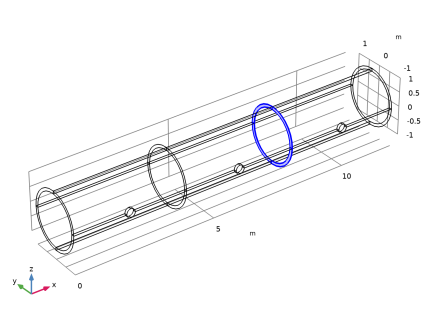
The right end of the Solid graph is connected to the left end of the Shell, Flexible graph at the flexible connection.

•

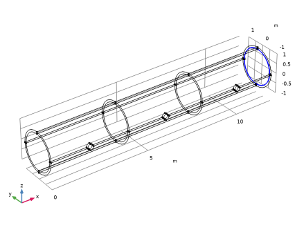
The right end of the Shell, Flexible graph is at the loaded end, where some local disturbances can appear.

From the graphs, it can be seen that:

Tension case

•

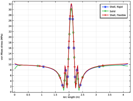
The correspondence between the solid and shell results are in general very good. This can be expected since the axial tension should give a homogeneous stress state in the undisturbed regions. At the hole edge, where stress gradients are steep, and three-dimensional effects important, there is a certain difference.

•

There is a disturbance in the results at both transitions between shell and solid, but it is more pronounced where the rigid formulation is used. The transition effect is seen only in the solid.

•

The details of the stresses in the transition can be seen in Figure 6 and Figure 7. In the latter figure it is clear that the flexible condition can describe the fact that the transverse stress should be zero much better than the rigid counterpart. The small bending stress seen also for the flexible connection depends on the fact that there is actually somewhat less material inside of the midsurface than it is outside of it. For a flat transition it would disappear almost completely.

Torsion case

•

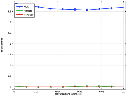
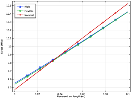
There is a general difference between the stress level in the shell and in the solid. The shell solution overestimates the through-thickness gradient of the shear stress somewhat. This is not related to the mixture of element types.

•

No transition effects can be seen. This is expected, since the stress state is pure shear in the plane of the shell. There are no transverse strains, so the same strain state should be possible to represent by both element types without extra assumptions.

•

The stress at the transitions is shown in Figure 8. The nominal stress level is the theoretical value. The linear through-thickness distribution is predicted by the torsion theory, and the equivalent stress shows no influence of other stress components than the shear stress.

Pressure case

•

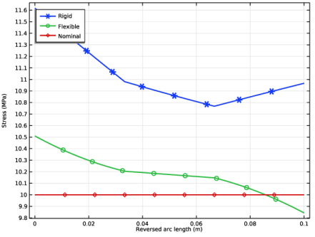
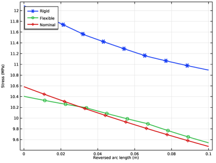
Also in this case, there is a difference in level between the shell solution and the solid solution. In the shell, only the midsurface stress is represented, whereas the solid can resolve the gradient in the thickness direction.

•

The transition effects are rather small, but approximately of the same size at both transitions. The stress state is predominantly a direct stress in the circumferential direction.

•

The hoop stress at the transitions is shown in Figure 9. The nominal value represents the theoretical value. It can be seen that the predictions using the flexible connection are significantly better than when using the rigid connection.

Figure 3: The von Mises stress plotted along the top of the pipe for the tension load case.

Figure 4: The von Mises stress plotted along the top of the pipe for the torsion load case.

Figure 5: The von Mises stress plotted along the top of the pipe for the pressure load case.

Figure 6: Axial stress through the thickness at the transitions (tension).

Figure 7: Transverse stress through the thickness at the transitions (tension).

Figure 8: Equivalent stress through the thickness at the transitions (torsion).

Figure 9: Hoop stress through the thickness at the transitions (pressure).

Structural_Mechanics_Module/Beams_and_Shells/shell_solid_connection

Modeling Instructions

From the menu, choose .

New

In the window, click

Model Wizard

In the window, click

In the tree, select .

Click .

In the tree, select .

Click .

Click

In the tree, select .

Click

Global Definitions

Define Parameters and Load Groups for use in the model setup.

Parameters 1

In the window, under click .

In the window for , locate the section.

Click

Browse to the model’s Application Libraries folder and double-click the file shell_solid_connection_parameters.txt.

Load Group, Tension

In the window, right-click and choose .

In the window for , type Load Group, Tension in the text field.

In the text field, type lgFx.

Load Group, Torsion

In the window, right-click and choose .

In the window for , type Load Group, Torsion in the text field.

In the text field, type lgMx.

Load Group, Pressure

Right-click and choose .

In the window for , type Load Group, Pressure in the text field.

In the text field, type lgP.

Geometry 1

Build the geometry by creating an array of three solid cylindrical parts with a cutout.

Cylinder 1 (cyl1)

In the toolbar, click

In the window for , locate the section.

In the text field, type r_outer.

In the text field, type length.

Locate the section. From the list, choose .

Click to expand the section. In the table, enter the following settings:


Layer name	Thickness (m)
Layer 1	thickness

Click

Delete Entities 1 (del1)

In the toolbar, click

In the window for , locate the section.

From the list, choose .

On the object , select Domain 3 only.

Click

Cylinder 2 (cyl2)

In the toolbar, click

In the window for , locate the section.

In the text field, type r_hole.

In the text field, type 1.5*r_outer.

Locate the section. In the text field, type length/2.

In the text field, type -1.5*r_outer.

Locate the section. From the list, choose .

Click

Difference 1 (dif1)

In the toolbar, click

and choose .

Select the object only.

In the window for , locate the section.

Find the subsection. Click to select the

toggle button.

Select the object only.

Click

Array 1 (arr1)

In the toolbar, click

and choose .

Select the object only.

In the window for , locate the section.

In the text field, type 3.

Locate the section. In the text field, type length.

Click

Click the

button in the toolbar.

Definitions

Create for various boundary and edge groups. It is easier selecting geometric entities using the wireframe rendering.

Click the

button in the toolbar.

Shell

In the toolbar, click

In the window for , type Shell in the text field.

Locate the section. From the list, choose .

Select Boundaries 6, 7, 11, 14, 48, 49, 53, and 56 only.

Solid

In the toolbar, click

In the window for , type Solid in the text field.

Select Domains 5–8 only.

Edges for Rigid Connection

In the toolbar, click

The option enables the selection of contiguous boundaries and edges with just one click.

In the window for , type Edges for Rigid Connection in the text field.

Locate the section. From the list, choose .

Select the check box.

Select Edges 39, 40, 45, and 48 only.

Edges for Flexible Connection

In the toolbar, click

In the window for , type Edges for Flexible Connection in the text field.

Locate the section. From the list, choose .

Select the check box.

Select Edges 73, 74, 79, and 82 only.

Boundaries for Rigid Connection

In the toolbar, click

In the window for , type Boundaries for Rigid Connection in the text field.

Locate the section. From the list, choose .

Select the check box.

Select Boundaries 22, 23, 29, and 33 only.

Boundaries for Flexible Connection

In the toolbar, click

In the window for , type Boundaries for Flexible Connection in the text field.

Locate the section. From the list, choose .

Select the check box.

Select Boundaries 43, 44, 50, and 54 only.

Constrained Edges

In the toolbar, click

In the window for , type Constrained Edges in the text field.

Locate the section. From the list, choose .

Click the

button in the toolbar.

Select the check box.

Select Edges 5, 6, 11, and 14 only.

Loaded Edges

In the toolbar, click

In the window for , type Loaded Edges in the text field.

Locate the section. From the list, choose .

Select the check box.

Select Edges 106, 107, 110, and 112 only.

Solid Inside

In the toolbar, click

In the window for , type Solid Inside in the text field.

Locate the section. From the list, choose .

Select Boundaries 27, 28, 32, and 35 only.

Solid Hole

In the toolbar, click

In the window for , type Solid Hole in the text field.

Locate the section. From the list, choose .

Select the check box.

Select Boundaries 38–41 only.

Shell Hole Edges

In the toolbar, click

In the window for , type Shell Hole Edges in the text field.

Locate the section. From the list, choose .

Select the check box.

Select Edges 24, 25, 30, 31, 92, 93, 98, and 99 only.

Click the

button in the toolbar.

Cylindrical System 2 (sys2)

In the toolbar, click

and choose .

You will use this cylindrical coordinate system for the definition of constraint and the torsional load.

In the window for , locate the section.

Find the subsection. In the table, enter the following settings:


x	y	z
1	0	0

Find the φ subsection. In the table, enter the following settings:


x	y	z
0	1	0

Since both the and parts use the same material data, start by adding Structural Steel as a global material and then use material links at domain and boundary levels.

Add Material

In the toolbar, click