You are viewing the documentation for an older COMSOL version. The latest version is available here.
PDF

Postbuckling Analysis of a Hinged Cylindrical Shell
Introduction
Buckling is a phenomenon that can cause sudden failure of a structure.
A linear buckling analysis predicts the critical buckling load. Such an analysis, however, does not give any information about what happens at loads higher than the critical load. Tracing the solution after the critical load is called a postbuckling analysis.
A linear buckling analysis also often overpredicts the load-carrying capacity of the structure.
In order to accurately determine the critical buckling load or predict the postbuckling behavior, you can use the nonlinear solver and ramp up the applied load to compute the structure deformation. The buckling load can then be based on when a certain, not acceptable, deformation is reached.
Once the critical buckling load has been reached it can happen that the structure undergoes a sudden large deformation into a new stable configuration. This is known as a snap-through phenomenon. A snap-through process cannot be simulated using prescribed load in a standard nonlinear static solver because the problem becomes numerically singular. Physically speaking, it is a highly transient problem as the structure “jumps” from one state to another. For simple cases with a single point load, it is often possible to replace the point load with a prescribed displacement and then measure the reaction force instead.
For more general problems the post-buckling solution must however be tracked using more sophisticated methods, as shown in this example.
Figure 1 shows the variation of load versus the displacement for such a difficult case. It illustrates the possible computational problem by using either a load control (path A) or a displacement control (path B).
Figure 1: Load versus displacement in snap-through buckling
The shell structure in this example has a behavior similar to this.
Model Definition
The model studied here is a benchmark for a hinged cylindrical panel subjected to a point load at its center; see Ref. 1.
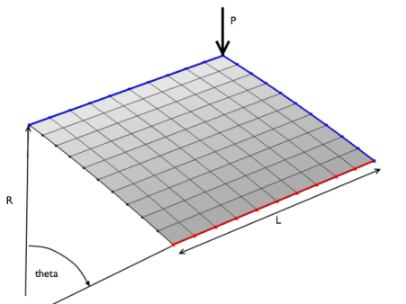
The radius of the cylinder is R = 2.54 m and all edges have a length of 2L = 0.508 m. The angular span of the panel is thus 0.2 radians. The panel thickness is th = 6.35 mm.
Due to the double symmetry, only one quarter of the geometry is modeled as shown in Figure 2. The blue lines show the symmetry edge conditions, while the red line shows the location of the hinged edge condition.
Figure 2: Problem description.
In general, you should be careful with using symmetry in buckling problems, because nonsymmetric solutions may exist.
Results
In Figure 3 you can see the applied load as a function of the panel center displacement. The figure shows clearly a non-unique solution for a given applied load (between -400 N to 600 N) or a given displacement (between 14.4 mm and 17 mm).
Figure 3: Applied load versus panel center displacement.
As shown in Table 1, the results agree well with the target data from Ref. 1.
Notes About the COMSOL Implementation
The main feature of this model is that a limit point instability occurs at the buckling load. Neither a load control, nor a point displacement control, would be able to track the jump between the stable solution paths (see Figure 1). To solve this type of problem it is important to find a proper parameter that increases monotonically.
In this example, a good such parameter is the average of the displacement in the direction of the applied force. You use a nonlocal average coupling to measure the displacement and then add a global equation to compute the appropriate point load for each prescribed parameter value.
There is no general way to determine which controlling parameter to use, so it is necessary to use some physical insight.
Reference
1. K.Y. Sze, X.H. Liua, and S.H. Lob, “Popular Benchmark Problems for Geometric Nonlinear Analysis of Shells,” Finite Element in Analysis and Design, vol. 40, issue 11, pp. 1551–1569, 2004.
Application Library path: Structural_Mechanics_Module/Verification_Examples/postbuckling_shell
Modeling Instructions
From the File menu, choose New.
New
In the New window, click  Model Wizard.
Model Wizard
1
In the Model Wizard window, click  3D.
2
In the Select Physics tree, select Structural Mechanics>Shell (shell).
3
Click Add.
4
Click  Study.
5
In the Select Study tree, select General Studies>Stationary.
6
Global Definitions
Parameters 1
1
In the Model Builder window, under Global Definitions click Parameters 1.
2
In the Settings window for Parameters, locate the Parameters section.
3
Geometry 1
Work Plane 1 (wp1)
1
In the Geometry toolbar, click  Work Plane.
2
In the Settings window for Work Plane, locate the Plane Definition section.
3
From the Plane list, choose xz-plane.
4
Click  Show Work Plane.
Work Plane 1 (wp1)>Line Segment 1 (ls1)
1
In the Work Plane toolbar, click  More Primitives and choose Line Segment.
2
In the Settings window for Line Segment, locate the Starting Point section.
3
From the Specify list, choose Coordinates.
4
Locate the Endpoint section. From the Specify list, choose Coordinates.
5
Locate the Starting Point section. In the yw text field, type R.
6
Locate the Endpoint section. In the xw text field, type L and yw to R.
7
Click  Build Selected.
Revolve 1 (rev1)
1
In the Model Builder window, right-click Geometry 1 and choose Revolve.
2
In the Settings window for Revolve, locate the Revolution Angles section.
3
Click the Angles button.
4
In the End angle text field, type theta.
5
Locate the Revolution Axis section. Find the Direction of revolution axis subsection. In the xw text field, type 1.
6
In the yw text field, type 0.
7
Click  Build Selected.
Definitions
Click the  Zoom Extents button in the Graphics toolbar.
Average 1 (aveop1)
1
In the Definitions toolbar, click  Nonlocal Couplings and choose Average.
2
In the Settings window for Average, locate the Source Selection section.
3
From the Geometric entity level list, choose Boundary.
4
Integration 1 (intop1)
1
In the Definitions toolbar, click  Nonlocal Couplings and choose Integration.
2
In the Settings window for Integration, locate the Source Selection section.
3
From the Geometric entity level list, choose Point.
4
Variables 1
1
In the Definitions toolbar, click  Local Variables.
2
In the Settings window for Variables, locate the Variables section.
3
Shell (shell)
Thickness and Offset 1
1
In the Model Builder window, under Component 1 (comp1)>Shell (shell) click Thickness and Offset 1.
2
In the Settings window for Thickness and Offset, locate the Thickness and Offset section.
3
In the d0 text field, type thic.
Symmetry 1
1
In the Physics toolbar, click  Edges and choose Symmetry.
2
Symmetry 2
1
In the Physics toolbar, click  Edges and choose Symmetry.
2
3
In the Settings window for Symmetry, locate the Coordinate System Selection section.
4
From the Coordinate system list, choose Global coordinate system.
5
Locate the Symmetry section. From the Symmetry plane normal list, choose First axis.
Pinned 1
1
In the Physics toolbar, click  Edges and choose Pinned.
2
Point Load 1
1
In the Physics toolbar, click  Points and choose Point Load.
2
Apply 1/4th of the total load because of the double symmetry used in this model.
3
In the Settings window for Point Load, locate the Force section.
4
Specify the FP vector as
5
Click the  Show More Options button in the Model Builder toolbar.
6
In the Show More Options dialog box, in the tree, select the check box for the node Physics>Equation-Based Contributions.
7
Global Equations 1
1
In the Physics toolbar, click  Global and choose Global Equations.
2
In the Settings window for Global Equations, locate the Global Equations section.
3
4
Locate the Units section. Click  Select Dependent Variable Quantity.
5
In the Physical Quantity dialog box, type force in the text field.
6
Click  Filter.
7
In the tree, select General>Force (N).
8
9
In the Settings window for Global Equations, locate the Units section.
10
Click  Select Source Term Quantity.
11
In the Physical Quantity dialog box, type displacement in the text field.
12
Click  Filter.
13
In the tree, select General>Displacement (m).
14
Materials
Material 1 (mat1)
1
In the Model Builder window, under Component 1 (comp1) right-click Materials and choose Blank Material.
2
In the Settings window for Material, locate the Material Contents section.
3
Mesh 1
Mapped 1
1
In the Mesh toolbar, click  Boundary and choose Mapped.
2
Distribution 1
1
Right-click Mapped 1 and choose Distribution.
2
3
In the Settings window for Distribution, locate the Distribution section.
4
In the Number of elements text field, type 10.
5
Click  Build Selected.
Study 1
Step 1: Stationary
Set up an auxiliary continuation sweep for the disp parameter.
1
In the Model Builder window, under Study 1 click Step 1: Stationary.
2
In the Settings window for Stationary, click to expand the Study Extensions section.
3
Select the Auxiliary sweep check box.
4
5
6
Locate the Study Settings section. Select the Include geometric nonlinearity check box.
Sometimes it is not straightforward to guess the maximum value of the parameter used. You can then instead set a stop condition for the parametric solver based on something that is known.
Solution 1 (sol1)
1
In the Study toolbar, click  Show Default Solver.
2
In the Model Builder window, expand the Solution 1 (sol1) node.
3
In the Model Builder window, expand the Study 1>Solver Configurations>Solution 1 (sol1)>Stationary Solver 1 node.
4
Right-click Study 1>Solver Configurations>Solution 1 (sol1)>Stationary Solver 1>Parametric 1 and choose Stop Condition.
5
In the Settings window for Stop Condition, locate the Stop Expressions section.
6
7
Specify that the solution is to be stored just before the stop condition is reached.
8
Locate the Output at Stop section. From the Add solution list, choose Step before stop.
9
Clear the Add warning check box.
10
In the Model Builder window, under Study 1>Solver Configurations>Solution 1 (sol1) click Stationary Solver 1.
11
In the Settings window for Stationary Solver, click to expand the Output section.
12
Clear the Reaction forces check box.
13
Click  Compute.
Results
Force at Shell Center
1
In the Home toolbar, click  Add Plot Group and choose 1D Plot Group.
2
In the Settings window for 1D Plot Group, type Force at Shell Center in the Label text field.
Point Graph 1
1
Right-click Force at Shell Center and choose Point Graph.
2
3
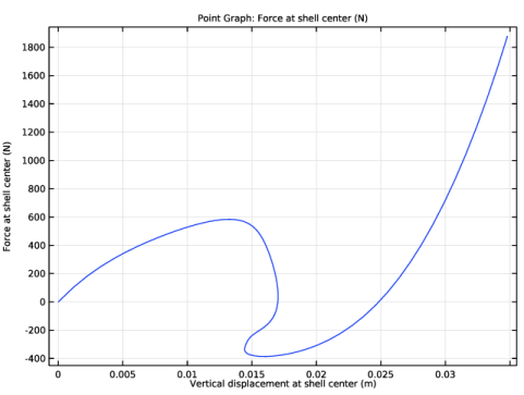
In the Settings window for Point Graph, click Replace Expression in the upper-right corner of the y-Axis Data section. From the menu, choose Component 1 (comp1)>Shell>P - Force at shell center - N.
4
Locate the x-Axis Data section. From the Parameter list, choose Expression.
5
In the Expression text field, type w_center.
6
In the Force at Shell Center toolbar, click  Plot.