Coupled Analysis of Flow and Stress in a Pipe

In this tutorial model, the flow in a pipe with a bend is computed using the Pipe Flow interface. The computed fluid load is used as input to a stress analysis in the Pipe Mechanics interface. Gravity loads from the pipe and fluid are also taken into account.

Model Definition

A circular pipe with outer diameter do = 10 cm consists of two straight 8 m long sections that are connected by a smooth 90-degree circular bend with a radius rb = 2 m; see Figure 1.

Figure 1: Pipe geometry.

Both ends are fixed, and the pipe is placed on three evenly spaced vertical supports.

The pipe wall thickness is t = 4 mm, so that the inner diameter is di = 9.2 cm. The inlet and outlet pressure are kept at 50 bar and 40 bar, respectively. A stationary flow of water in the pipe is driven by the resulting pressure drop. The pressure outside the pipe is assumed to be negligible. Thus, a significant internal overpressure, p, causes a hoop stress in the pipe walls.

The pipe is made of steel and has the inner surface roughness of e = 0.046 mm.

The system is subjected to the gravity, so that the pipe and fluid weight causes the pipe vertical bending. In addition, the flow acts on the pipe in two ways: the drag force due to the wall friction, and the centrifugal force in the bend. Both forces lead to the pipe horizontal deflection and bending.

The drag force acts along the pipe and is estimated using the Swamee-Jain formula (Ref. 1)

which is valid for relative roughness 1·10−6 < e/di < 1·10−2 and 5·103 < Re < 1·108. The Reynolds number is Re = ρudi/μ, where u is the flow velocity, ρ is water density, and μ is the dynamic viscosity.

The centrifugal force acts outward the bend perpendicular to the pipe, and its magnitude is given by: ρAu2/rb, where A is the area of the pipe inner cross section.

Results and Discussion

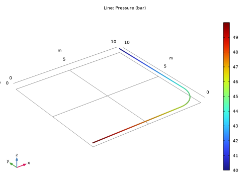
The pressure distribution inside the pipe is shown in Figure 2. The flow has a uniform velocity around 23.8 m/s along the whole pipe, which corresponds to the Reynolds number Re = 2.2·106 that indicates that the flow regime is highly turbulent.

Figure 2: Pressure distribution.

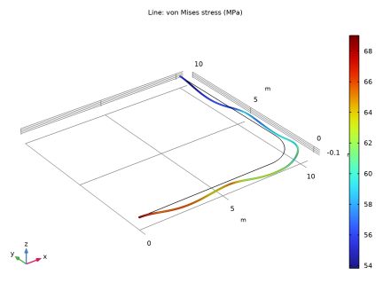
The stress distribution in the pipe walls is shown in Figure 3. Due to the pressure drop in the fluid, the value is higher at the inlet than at the outlet. The pipe displacement components are shown in Figure 4. The importance of the vertical supports is clearly visible.

Figure 3: von Mises stress distribution along the deformed pipe.The deformation is scaled by approximately a factor of 150.

Figure 4: Pipe displacement.

The bending moments and shear forces along the pipe are shown in Figure 5 and Figure 6.

Figure 5: Bending moments.

Figure 6: Shear forces.

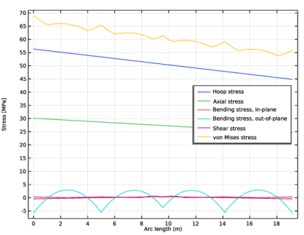
The different contributions to the total stress state are shown in Figure 7. As is common in piping systems, the hoop stress caused by the internal pressure is dominant.

Figure 7: Stress contributions.

Notes About the COMSOL Implementation

You start the model setup by adding a multiphysics interface Fluid-Pipe Interaction, Fixed Geometry. This will bring in two physics interfaces, Pipe Flow and Pipe Mechanics, together with a multiphysics coupling feature Fluid-Pipe Interaction.

The interfaces are one-way coupled. Thus, the flow will affect the structural displacement, but the pipe geometry change because of the deformation is assumed to be small and will have no effect on the flow computations.

The flow induced forces such as internal overpressure, drag and centrifugal forces are computed and applied on the structure automatically by the coupling feature.

The Pipe Mechanics interface needs two materials, one for the pipe wall and the other for the contained fluid. The materials are chosen in the node under the interface. The material selection lists will contain all materials available in the component. The material data will be taken from the selected material even if the corresponding material node has no selection or is overridden under in the component. The interface can only take data from an active material with proper selection made under in the component.

Reference

1. P.K Swamee and A.K. Jain, “Explicit Equations for Pipe-flow Problems”, J. Hydraulics Division (ASCE), vol. 102, no. 5, pp. 657–664, 1976.

Structural_Mechanics_Module/Pipe_Mechanics/pipe_flow_stress

Modeling Instructions

From the menu, choose .

New

In the window, click