PDF

Peristaltic Pump
Introduction
In a peristaltic pump, rotating rollers squeeze a flexible tube. As the pushed-down rollers move along the tube, fluids in the tube follow the motion. The main advantage of the peristaltic pump is that no seals, valves, or other internal parts ever touch the fluid. Due to their cleanliness, peristaltic pumps have found many applications in the pharmaceutical, chemical, and food industries. Besides this, the action of a peristaltic pump is very gentle, which is important if the fluid can be easily damaged. Peristaltic pumps are therefore used in medical applications, one of which is to move the blood through the body during open heart surgery. Other types of pumps would risk destroying the blood cells.
In this COMSOL Multiphysics example, a peristaltic pump is analyzed by combining structural mechanics (to model the squeezing of the tube) and fluid dynamics (to compute the fluid’s motion). Thus, it is an example of a fluid-structure interaction (FSI) problem.
Model Definition
The analysis is set up in 2D axial symmetry (Figure 1). A nylon tube 0.1 m long has an inner radius of 1 cm and an outer radius of 1.5 cm; it contains fluid with the density ρ = 1·103 kg/m3 and viscosity μ = 5·103 Pa·s. A time- and position-dependent force density is applied to the outer wall of the tube, in the radial direction. This force density could have been taken from real data from a peristaltic pump operation. For the sake of simplicity, this example models it with a Gaussian distribution along the length of the tube. The Gaussian distribution has a width of 1 cm and is moving with the constant velocity 0.03 m/s in the positive z direction. To represent the engagement of the roll, the force density, multiplied by a smoothed Heaviside function, kicks in at t = 0.1 s and takes the force to its full development at t = 0.5 s. Likewise, the disengagement of the roll starts at t = 1.0 s and ends at t = 1.4 s. The example models the tube’s deformation during a full cycle of 1.5 s.
Figure 1: The geometry of the peristaltic pump as it is deforming under the pressure of the roll. The tube is rotationally symmetric with respect to the z-axis. The color shows the deformation of the tube material.
Domain Equations
The structural mechanics computations use the assumption that the material is linear elastic, and they take geometric nonlinearities into account.
The fluid flow is described by the incompressible Navier-Stokes equations:
where ρ denotes the density (SI unit: kg/m3), u the velocity (SI unit: m/s), μ the viscosity (SI unit: Pa·s), and p the pressure (SI unit: Pa). The equations are set up and solved inside the tube.
The Navier-Stokes equations are solved on a freely moving deformed mesh, which constitutes the fluid domain. The deformation of this mesh relative to the initial shape of the domain is computed using Hyperelastic smoothing. On the solid-fluid boundary at the tube’s inner wall, the moving mesh follows the structural deformation. For more information, please refer to the chapter Fluid-Structure Interaction in the Structural Mechanics Module User’s Guide.
Boundary Conditions
For the structural mechanics computations, the time- and coordinate-dependent load is prescribed as the boundary condition at the tube’s outer surface. This is the load that drives the pump operation. The top and bottom ends of the tube are constrained along both coordinate axes.
For the fluid simulation, the boundary condition at the inlet and the outlet assumes that the total stress is zero, that is:
The mesh has zero z displacement at the top and the bottom of the tube.
At the fluid-solid boundary, the structural velocity is transmitted to the fluid. As a feedback, the stresses in the fluid flow act as a loading on the inner boundary of the solid wall of the tube.
Computation of Volumetric Flow Rates and Total Volume of Pumped Fluid
The model’s dependent variables are the displacements of the tube wall together with the fluid velocity u = (u, v) and pressure p.
To get the volumetric flow rate of the fluid in m3/s and the total volume of pumped fluid, you need to perform some additional calculations. To obtain the volumetric flow rate at any instant t, compute a boundary integral over the pipe’s inlet and outlet boundary:
where n is the outward-pointing unit normal of the boundary, u is the velocity vector, and s is the boundary length parameter, along which you integrate. In this particular model, the inlet and outlet boundaries are horizontal so n · u = nxu + nyv simplifies to v or v depending on the direction of the flow.
It is of interest to track how much fluid is conveyed through the outlet during a peristaltic cycle, This can be calculated as the following time integral:
To compute this integral, specify the corresponding ODE in COMSOL Multiphysics
with proper initial conditions; the software then will integrate this equation.
Results
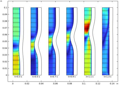
Figure 2 shows several snapshots from the peristaltic pump in action.
Figure 2: Snapshots of the velocity field and the shape of the inside of the tube at different times. The colors represent the magnitude of the velocity, and the arrows its direction.
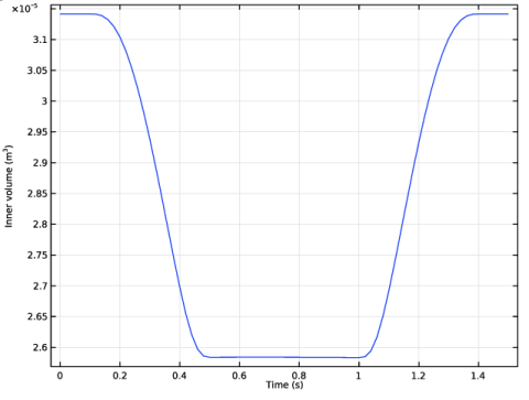
Figure 3 shows the inner volume of the tube as a function of time. At t = 0.3 s, the roll has begun its engagement phase, and it is increasing its pressure on the tube. As less and less space is left for the fluid, it is streaming out of the tube, through both the inlet and the outlet. At0.5 s, the roll has been fully engaged for a while. As it is moving upward along the tube, so does the fluid, both at the inlet and at the outlet. This is where most of the net flow in the direction from the inlet to the outlet is created. Finally, at t = 1.3 s, the engagement process is reversed, and the roll is disengaging. As a result, the fluid is streaming into the tube from both ends.
Figure 3: The inner volume (m3) of the tube as a function of time (s).
Figure 4 shows the inlet and outlet flows, and it confirms the overall behavior indicated in the velocity snapshots. Note that a real peristaltic pump usually removes or minimizes the peaks associated with volume changes with the help of a second roll that engages at the same time as the first roll disengages. This way, there are hardly any volume changes, and the fluid flows forward all the time. Also note from Figure 4 that by taking the difference of the curves, and integrating over time, you generate Figure 3.
Figure 4: Inlet and outlet flow in m3/s as functions of time. Positive values indicate that the fluid is flowing in through the inlet and out through the outlet.
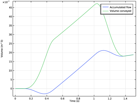
Figure 5 sums up the process, plotting the accumulated net flow versus time. It is worth noting that although the accumulated flow during the first 0.5 s of the cycle is zero or negative, it is well above zero after the full cycle.
Figure 5: Accumulated flow (m3) through the pump and volume of fluid conveyed out of the outlet versus time (s).
Notes About the COMSOL Implementation
This example is primarily intended to demonstrate the use of the Fluid-Structure Interaction multiphysics coupling, but it also shows some features for results analysis. Thus, it defines integration coupling operators to calculate the flow rate. An ordinary differential equation is used for calculating the accumulated fluid volume that has passed through the pump at certain points in time. The smooth step function used in this example is called flc2hs (a C2-continuous step).
Application Library path: Structural_Mechanics_Module/Fluid-Structure_Interaction/peristaltic_pump
Modeling Instructions
From the File menu, choose New.
New
In the New window, click  Model Wizard.
Model Wizard
1
In the Model Wizard window, click  2D Axisymmetric.
2
In the Select Physics tree, select Fluid Flow>Fluid-Structure Interaction>Fluid-Solid Interaction.
3
Click Add.
4
Click  Study.
5
In the Select Study tree, select General Studies>Time Dependent.
6
Geometry 1
Rectangle 1 (r1)
1
In the Geometry toolbar, click  Rectangle.
2
In the Settings window for Rectangle, locate the Size and Shape section.
3
In the Width text field, type 0.01.
4
In the Height text field, type 0.1.
5
Click  Build All Objects.
Rectangle 2 (r2)
1
In the Geometry toolbar, click  Rectangle.
2
In the Settings window for Rectangle, locate the Size and Shape section.
3
In the Width text field, type 5e-3.
4
In the Height text field, type 0.1.
5
Locate the Position section. In the r text field, type 0.01.
6
Click  Build All Objects.
Global Definitions
Parameters 1
1
In the Model Builder window, under Global Definitions click Parameters 1.
2
In the Settings window for Parameters, locate the Parameters section.
3
Definitions
Follow the steps given below to define the force density of the load applied to the outer wall of the tube.
Analytic 1 (an1)
1
In the Home toolbar, click  Functions and choose Local>Analytic.
2
In the Settings window for Analytic, type load in the Function name text field.
3
Locate the Definition section. In the Expression text field, type flc2hs(t_off/dt-ts,1)*flc2hs(ts-t_on/dt,1)*exp(-(zs-(z0+v0*ts*dt)/width)^2/2).
4
In the Arguments text field, type zs,ts.
Note that the function arguments are made dimensionless by zs = z/width and ts = t/dt.
To compute inflow/outflow rates, define the integration over the relevant boundaries.
Integration 1 (intop1)
1
In the Definitions toolbar, click  Nonlocal Couplings and choose Integration.
2
In the Settings window for Integration, locate the Source Selection section.
3
From the Geometric entity level list, choose Boundary.
4
5
Locate the Advanced section. Clear the Compute integral in revolved geometry check box.
Integration 2 (intop2)
1
In the Definitions toolbar, click  Nonlocal Couplings and choose Integration.
2
In the Settings window for Integration, locate the Source Selection section.
3
From the Geometric entity level list, choose Boundary.
4
5
Locate the Advanced section. Clear the Compute integral in revolved geometry check box.
Variables 1
1
In the Definitions toolbar, click  Local Variables.
2
In the Settings window for Variables, locate the Variables section.
3
Moving Mesh
Deforming Domain 1
1
In the Model Builder window, under Component 1 (comp1)>Moving Mesh click Deforming Domain 1.
2
Laminar Flow (spf)
1
In the Model Builder window, under Component 1 (comp1) click Laminar Flow (spf).
2
Open Boundary 1
1
In the Physics toolbar, click  Boundaries and choose Open Boundary.
2
Define the ordinary differential equations to calculate the volume of the pumped fluid and the accumulated flow.
3
Click the  Show More Options button in the Model Builder toolbar.
4
In the Show More Options dialog box, in the tree, select the check box for the node Physics>Equation-Based Contributions.
5
Global Equations 1
1
In the Physics toolbar, click  Global and choose Global Equations.
2
In the Settings window for Global Equations, locate the Global Equations section.
3
4
Locate the Units section. Click  Select Dependent Variable Quantity.
5
In the Physical Quantity dialog box, type volume in the text field.
6
Click  Filter.
7
In the tree, select General>Volume (m^3).
8
9
In the Settings window for Global Equations, locate the Units section.
10
Click  Select Source Term Quantity.
11
In the Physical Quantity dialog box, type volumepertime in the text field.
12
Click  Filter.
13
In the tree, select General>Volume per time (m^3/s).
14
Global Equations 2
1
In the Physics toolbar, click  Global and choose Global Equations.
2
In the Settings window for Global Equations, locate the Global Equations section.
3
4
Locate the Units section. Click  Select Dependent Variable Quantity.
5
In the Physical Quantity dialog box, type volume in the text field.
6
Click  Filter.
7
In the tree, select General>Volume (m^3).
8
9
In the Settings window for Global Equations, locate the Units section.
10
Click  Select Source Term Quantity.
11
In the Physical Quantity dialog box, type volumepertime in the text field.
12
Click  Filter.
13
In the tree, select General>Volume per time (m^3/s).
14
Solid Mechanics (solid)
1
In the Model Builder window, under Component 1 (comp1) click Solid Mechanics (solid).
2
Linear Elastic Material 1
In the Model Builder window, under Component 1 (comp1)>Solid Mechanics (solid) click Linear Elastic Material 1.
Damping 1
1
In the Physics toolbar, click  Attributes and choose Damping.
2
In the Settings window for Damping, locate the Damping Settings section.
3
In the αdM text field, type 1e-2.
4
In the βdK text field, type 1e-3.
Fixed Constraint 1
1
In the Physics toolbar, click  Boundaries and choose Fixed Constraint.
2
Boundary Load 1
1
In the Physics toolbar, click  Boundaries and choose Boundary Load.
2
3
In the Settings window for Boundary Load, locate the Force section.
4
Specify the FA vector as
Component 1 (comp1)
Symmetry/Roller 1
1
In the Definitions toolbar, click  Moving Mesh and choose Boundaries>Symmetry/Roller.
2
Add Material
1
In the Home toolbar, click  Add Material to open the Add Material window.
2
Go to the Add Material window.
3
In the tree, select Built-in>Nylon.
4
Click Add to Component in the window toolbar.
5
In the Home toolbar, click  Add Material to close the Add Material window.
Materials
Nylon (mat1)
1
In the Settings window for Material, locate the Geometric Entity Selection section.
2
From the Selection list, choose Manual.
3
Material 2 (mat2)
1
In the Model Builder window, right-click Materials and choose Blank Material.
2
3
In the Settings window for Material, locate the Material Contents section.
4
Study 1
Step 1: Time Dependent
1
In the Model Builder window, under Study 1 click Step 1: Time Dependent.
2
In the Settings window for Time Dependent, locate the Study Settings section.
3
In the Output times text field, type range(0,0.02,1.5).
Get the initial values, which will also generate the default plot to be shown while solving.
4
Right-click Study 1>Step 1: Time Dependent and choose Get Initial Value for Step.
Study 1
Step 1: Time Dependent
1
In the Model Builder window, expand the Results>Datasets node, then click Study 1>Step 1: Time Dependent.
2
In the Settings window for Time Dependent, click to expand the Results While Solving section.
3
Select the Plot check box.
4
In the Home toolbar, click  Compute.
The first default plot shows the velocity field at t = 1.5 s. To plot the displacement at t = 0.7 s (Figure 1), add it from the predefined plots:
5
Click  Add Predefined Plot.
Add Predefined Plot
1
Go to the Add Predefined Plot window.
2
In the tree, select Study 1/Solution 1 (sol1)>Solid Mechanics>Displacement (solid).
3
Click Add Plot in the window toolbar.
4
In the Home toolbar, click  Add Predefined Plot.
Results
Displacement (solid)
1
In the Model Builder window, under Results click Displacement (solid).
2
In the Settings window for 2D Plot Group, locate the Data section.
3
From the Time (s) list, choose 0.7.
Surface 1
1
In the Model Builder window, expand the Displacement (solid) node, then click Surface 1.
2
In the Settings window for Surface, locate the Expression section.
3
From the Unit list, choose mm.
4
In the Displacement (solid) toolbar, click  Plot.
Velocity (spf)
Animate the velocity field as a function of time, as shown in Figure 2.
1
In the Model Builder window, under Results click Velocity (spf).
Animation 1
In the Velocity (spf) toolbar, click  Animation and choose Player.
Velocity (spf)
To plot the total volume of fluid contained in the pump (Figure 3), follow the steps given below.
Surface Measurement 1
1
In the Model Builder window, expand the Results>Velocity (spf) node.
2
Right-click Results>Derived Values and choose Measure>Surface Measurement.
3
4
In the Settings window for Surface Measurement, locate the Measurement Settings section.
5
Select the Description check box. In the associated text field, type Inner volume.
6
Click  Evaluate.
Table
1
Go to the Table window.
2
Click the right end of the Display Table 1 - Surface Measurement 1 split button in the window toolbar.
3
Results
Inner Volume
1
In the Model Builder window, under Results click 1D Plot Group 7.
2
In the Settings window for 1D Plot Group, type Inner Volume in the Label text field.
To plot the inlet and outlet flow rates (Figure 4), accumulated flow through the pump and volume of fluid conveyed out of the outlet(Figure 5), follow the steps given below.
Inflow and Outflow
1
In the Results toolbar, click  1D Plot Group.
2
In the Settings window for 1D Plot Group, type Inflow and Outflow in the Label text field.
3
Locate the Plot Settings section.
4
Select the y-axis label check box. In the associated text field, type Flow (m^3/s).
Global 1
1
Right-click Inflow and Outflow and choose Global.
2
In the Settings window for Global, locate the y-Axis Data section.
3
4
Click to expand the Title section. From the Title type list, choose None.
5
In the Inflow and Outflow toolbar, click  Plot.
Accumulated and Conveyed Flow
1
In the Home toolbar, click  Add Plot Group and choose 1D Plot Group.
2
In the Settings window for 1D Plot Group, type Accumulated and Conveyed Flow in the Label text field.
3
Locate the Plot Settings section.
4
Select the y-axis label check box. In the associated text field, type Volume (m^3).
Global 1
1
Right-click Accumulated and Conveyed Flow and choose Global.
2
In the Settings window for Global, locate the y-Axis Data section.
3
4
Locate the Title section. From the Title type list, choose None.
5
In the Accumulated and Conveyed Flow toolbar, click  Plot.
Flow and Stress, 3D
1
In the Model Builder window, under Results click Velocity, 3D (spf).
2
In the Settings window for 3D Plot Group, type Flow and Stress, 3D in the Label text field.
3
Locate the Data section. From the Time (s) list, choose 0.7.
Surface 2
1
Right-click Flow and Stress, 3D and choose Surface.
2
In the Settings window for Surface, locate the Expression section.
3
In the Expression text field, type solid.mises.
4
From the Unit list, choose MPa.
5
Locate the Coloring and Style section. Click  Change Color Table.
6
In the Color Table dialog box, select Rainbow>Prism in the tree.
7
8
In the Flow and Stress, 3D toolbar, click  Plot.
The resulting plot should be similar to the one shown in the following figure: