|
|
|


|
5.96·106 S/m
|
||
|
2·10-4
|
||
|
1.5·106 A/m
|

|
1
|
|
2
|
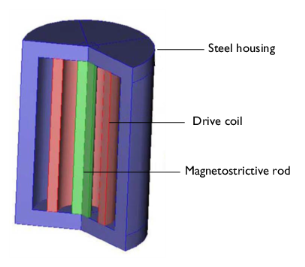
In the Select Physics tree, select Structural Mechanics>Electromagnetics-Structure Interaction>Magnetostriction>Nonlinear Magnetostriction.
|
|
3
|
Click Add.
|
|
4
|
Click
|
|
5
|
|
6
|
Click
|
|
1
|
|
2
|
|
3
|
|
1
|
|
2
|
|
3
|
|
4
|
|
5
|
|
6
|
|
1
|
|
2
|
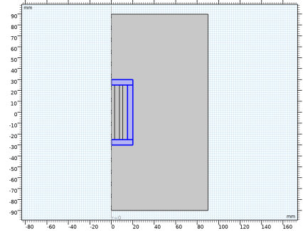
Select the object r1 only.
|
|
3
|
|
4
|
|
5
|
|
1
|
|
2
|
|
3
|
|
4
|
|
5
|
|
6
|
|
1
|
|
2
|
Select the object r2 only.
|
|
3
|
|
4
|
|
5
|
|
1
|
|
2
|
|
3
|
|
4
|
|
5
|
|
6
|
|
7
|
|
1
|
|
2
|
|
3
|
|
4
|
|
5
|
|
6
|
|
7
|
|
1
|
|
2
|
|
3
|
|
4
|
|
1
|
|
2
|
|
3
|
|
1
|
|
2
|
|
1
|
|
2
|
|
3
|
|
1
|
|
3
|
|
4
|
|
5
|
|
1
|
|
2
|
In the Settings window for Ampère’s Law, Nonlinear Magnetostrictive, locate the Domain Selection section.
|
|
3
|
|
4
|
|
1
|
|
3
|
|
4
|
|
1
|
|
2
|
|
3
|
In the tree, select Built-in>Air.
|
|
4
|
|
5
|
|
6
|
|
7
|
|
1
|
|
1
|
|
2
|
|
4
|
|
1
|
|
1
|
|
2
|
|
3
|
|
1
|
|
2
|
|
3
|
Click the Custom button.
|
|
4
|
|
5
|
|
1
|
|
2
|
|
1
|
|
2
|
|
3
|
|
4
|
|
5
|
|
6
|
|
7
|
Click
|
|
1
|
|
2
|
|
3
|
|
4
|
|
5
|
|
1
|
|
2
|
|
3
|
|
4
|
|
5
|
|
1
|
|
2
|
|
1
|
|
2
|
In the Settings window for Surface, click Replace Expression in the upper-right corner of the Expression section. From the menu, choose Component 1 (comp1)>Solid Mechanics>Strain>Strain tensor (material and geometry frames)>solid.eZZ - Strain tensor, ZZ-component.
|
|
3
|
|
1
|
|
2
|
|
3
|
|
4
|
|
5
|
Locate the Arrow Positioning section. Find the r grid points subsection. In the Points text field, type 20.
|
|
6
|
|
7
|
|
8
|
|
1
|
|
2
|
|
3
|
|
4
|
|
1
|
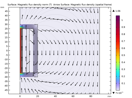
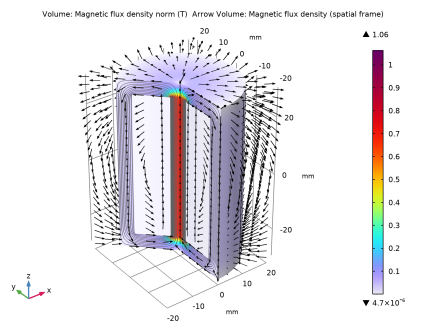
In the Model Builder window, under Results click Magnetic Flux Density Norm, Revolved Geometry (mf).
|
|
2
|
|
3
|
|
1
|
|
2
|
|
3
|
|
4
|
|
5
|
|
6
|
Locate the Arrow Positioning section. Find the x grid points subsection. From the Entry method list, choose Coordinates.
|
|
7
|
|
8
|
|
9
|
|
10
|
|
11
|
|
12
|
|
13
|
|
14
|
|
15
|
|
1
|
|
3
|
|
4
|
|
1
|
|
2
|
|
3
|
|
4
|
|
5
|
|
1
|
|
2
|
|
3
|
|
1
|
|
2
|
|
3
|
|
4
|
Click
|
|
5
|
|
6
|
Click
|
|
7
|
|
8
|
|
9
|
|
10
|
|
11
|
Click Add.
|
|
1
|
|
2
|
|
3
|
Click
|
|
5
|
|
1
|
|
2
|
|
3
|
|
4
|
|
5
|
|
6
|
|
7
|
|
8
|
|
9
|
|
1
|
|
2
|
|
3
|
|
4
|
|
5
|
Click OK.
|
|
6
|
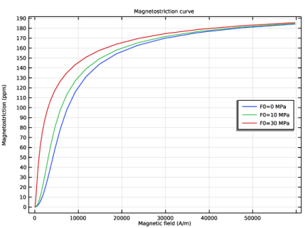
In the Settings window for Point Graph, click Replace Expression in the upper-right corner of the y-Axis Data section. From the menu, choose Component 1 (comp1)>Multiphysics>Strain>Magnetostrictive strain tensor>npzm1.emeZZ - Magnetostrictive strain tensor, ZZ-component.
|
|
7
|
|
8
|
|
9
|
Click Replace Expression in the upper-right corner of the x-Axis Data section. From the menu, choose Component 1 (comp1)>Magnetic Fields>Magnetic>Magnetic field (material and geometry frames) - A/m>mf.HZ - Magnetic field, Z-component.
|
|
10
|
|
11
|
|
12
|
|
1
|
|
2
|
|
3
|
|
4
|
|
1
|
|
2
|
In the Settings window for Point Graph, click Replace Expression in the upper-right corner of the y-Axis Data section. From the menu, choose Component 1 (comp1)>Magnetic Fields>Magnetic>Magnetic flux density (material and geometry frames) - T>mf.BZ - Magnetic flux density, Z-component.
|
|
3
|
|
1
|
|
2
|
|
3
|
|
4
|
|
5
|
|
6
|
|
7
|
|
8
|
|
9
|
|
1
|
|
2
|
|
3
|
|
4
|
|
5
|
Click OK.
|
|
6
|
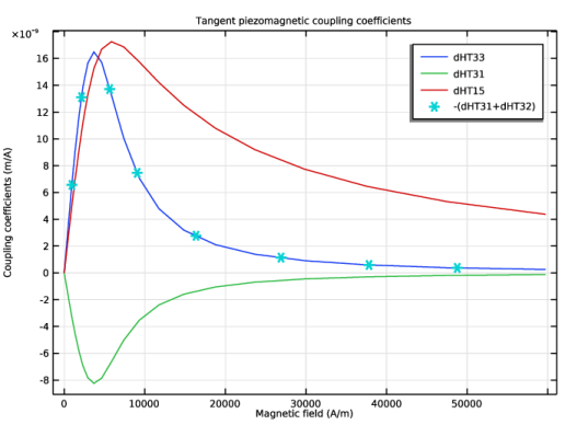
In the Settings window for Point Graph, click Replace Expression in the upper-right corner of the y-Axis Data section. From the menu, choose Component 1 (comp1)>Multiphysics>Effective properties>Tangent piezomagnetic coupling matrix, Voigt notation - m/A>npzm1.dHT33 - Tangent piezomagnetic coupling matrix, Voigt notation, 33-component.
|
|
7
|
|
8
|
|
9
|
|
10
|
|
1
|
|
2
|
|
3
|
|
4
|
Locate the Legends section. In the table, enter the following settings:
|
|
1
|
|
2
|
|
3
|
|
4
|
Locate the Legends section. In the table, enter the following settings:
|
|
1
|
|
2
|
|
3
|
|
4
|
Locate the Legends section. In the table, enter the following settings:
|
|
5
|
Click to expand the Coloring and Style section. Find the Line style subsection. From the Line list, choose None.
|
|
6
|
|
7
|
|
8
|