You are viewing the documentation for an older COMSOL version. The latest version is available here.
PDF

Random Vibration Test of a Motherboard
Introduction
Electronic components are often placed in an environment, where they will be subjected to vibrations. For many such components, it may be mandatory to perform vibration tests. The tests are performed by attaching the component to a shaker table, where it will be subjected to a pseudorandom acceleration. The acceleration input has a frequency content given by a specified power spectral density (PSD). The input is sometimes also called acceleration spectral density (ASD).
In order to predict the outcome of such a test, it is possible to perform a simulation using random vibration analysis. This example shows how such an analysis can be done.
The analyzed structure is a motherboard with some components attached.
Model Definition
GEOMETRY
Figure 1 shows a motherboard with a design that is typical for smaller computer devices such as game consoles, for example.
Figure 1: Motherboard geometry.
A processor (CPU) and a graphics chip (GPU) are covered by massive heat sinks used for passive cooling. Memory chips are located next to the CPU unit. A number of cylindrical capacitors of various sizes are scattered over the motherboard. Several connectors for peripherals are located along the motherboard’s edges. The board is intended to be attached to the housing via six mounting bolts. The latter are not modeled explicitly. The structure is attached to the shaker table during vibration testing at the same locations.
Material
The board itself is made of a generic PCB material. The heat sinks are made of aluminum. The chips are modeled as made of silicon. The connectors are modeled as rectangular blocks made of plastic. Some effective material properties are used to represent the capacitors.
Rayleigh damping is assumed, with a relative damping of 0.04 at the frequencies 40 and 1000 Hz.
Constraints
All six mounting holes are considered to be fixed to the shaker table. In order to be able to measure the bolt forces, rigid connectors are used instead of ordinary fixed constraints.
Loads
The loading is provided by an acceleration of the shaker table. The power spectral density for this test is shown in Figure 2. The test is performed three times, where the structure is independently accelerated in each of the three global directions. Thus, three different Random Vibration nodes are also used. The acceleration cannot be explicitly prescribed for a ground motion when a modal based study is used. Instead, the Base Excitation feature is used. It provides a uniform body force to the structure.
Figure 2: The power spectral density for the applied acceleration.
Mounting Bolts
The motherboard is designed to be mounted with six M3 bolts. The following properties are assumed:
Mounting prestress: 200 MPa (giving a bolt force of 1 kN)
Given these numbers, the maximum allowable shear force without sliding is  = 120 N.
Each bolt is modeled by a rigid connector constrained in all degrees of freedom (DOFs), so that it is possible to measure the individual reaction forces.
Mesh
Figure 3 shows the mesh used.
Figure 3: Mesh.
The discretization using this mesh together with quadratic serendipity elements results in approximately 100,000 DOFs being used in the eigenfrequency analysis.
Results and Discussion
The excitation PSD covers a large frequency range, 20 — 2000 Hz. As an effect, a large number of eigenfrequencies and corresponding eigenmodes (about 100) have to be computed. Using all these eigenmodes in the reduced-order model may however lead to long evaluation times. It is thus useful to investigate their relative importance. A good indicator is the modal mass. In Figure 4, the relative modal mass in each direction is shown for all eigenmodes.
Figure 4: The distribution of modal mass for all computed eigenmodes.
As can be seen, the relative modal mass can differ by orders of magnitude between different modes. In the analyses, only modes with a relative modal mass larger than 0.001 are included. It should however be noted that modes which mainly consists of the movement of a single small component can have a low value of the participation factor, so this type of truncation should be used with some care.
In Figure 5 to Figure 7, the RMS accelerations are plotted for each of the three excitation directions. One important note here, is that since the actual acceleration from the shaker table is transformed into an equivalent inertial force, all displacements, velocities, and accelerations are computed relative to the fixation points. While this often is relevant for displacements, you will in most cases be interested in the accelerations relative to a space-fixed frame (absolute accelerations). This is what would be measured by an attached accelerometer. To compute the PSD and RMS values for the absolute accelerations, the PSD of the excitation must be added. There are special built-in acceleration variables that take care of this transformation.
Figure 5: RMS of absolute acceleration caused by excitation in the X direction.
Figure 6: RMS of absolute acceleration caused by excitation in the Y direction.
Figure 7: RMS of absolute acceleration caused by excitation in the Z direction.
For the worst case (shown in Figure 6), the RMS acceleration in some of the capacitors reaches about 70g. Assuming that the peak value is three times larger than the RMS, the peak acceleration can be estimated to about 200g. This is a high value, so the allowed accelerations for the affected components should be checked.
In order to get a better understanding of how different parts of the spectrum contribute to the RMS value, it is instructive to plot the PSD at locations with high RMS values. In Figure 8 through Figure 10, the PSD is plotted as function of frequency for a point on top of one of the small capacitors showing large accelerations in Figure 6. You can clearly see how the input spectrum equals the output spectrum for the excitation direction at low frequencies.
Figure 8: Computed PSD of the absolute acceleration for one of the capacitors when subjected to X direction excitation.
Figure 9: Computed PSD of the absolute acceleration for one of the capacitors when subjected to Y direction excitation.
Figure 10: Computed PSD of the absolute acceleration for one of the capacitors when subjected to Z direction excitation.
Finally, the capacity of the mounting bolts are checked. In particular, the risk of sliding under the bolt heads is considered. Given the largest allowed shear force for a single bolt, , a margin of safety can be defined as
where the assumption that the peak value exceeds the RMS value by a factor of 3 has been introduced.
Tables of all bolt forces and corresponding margins of safety are generated in the Bolt Forces X-excitation, Bolt Forces Y-excitation, and Bolt Forces Z-excitation nodes under Derived Values. The margin is positive for all bolts, however it is rather small in all three excitation directions for the bolts labeled ‘Bolt 2’ and ‘Bolt 5’. The smallest value, for Z-direction excitation, is about 0.02.
If there is sliding under the bolt head, there is a risk that the bolt will lose its grip. If that would happen, the whole analysis would be invalidated, since the boundary conditions are no longer the same. The margin of safety is, however, determined with respect to the estimated peak value, so the force will not be that large for many load cycles. The bolts can thus be considered as validated.
Notes About the COMSOL Implementation
The given acceleration spectrum is that of the shaker table, that is what the bolt locations experience. The load is applied using a Base Excitation node. This is usually the preferred approach if all supports move synchronously, as is the case in vibration testing. Otherwise, the approximate large mass method must be used.
When computing the RMS value of the accelerations, the q2 and q2sq operators are used. These operators are similar to the rms operator, but act on a quadratic form. The simpler of these operators, q2sq, takes predefined variables defined for random vibration as input, and directly returns the RMS. When supplying user-defined quadratic forms, the q2 operator is used instead. This operator returns the square of the RMS. The following three cases would give the same result for a single variable u:
rvib1.rms(u,...)
sqrt(rvib1.q2(u^2,...)
rvib1.q2sq(sqrt(u^2+eps),...)
For the total relative displacement, the following cases are equivalent for computing the RMS:
rvib1.q2sq(solid.disp_rv,...)
sqrt(rvib1.q2(u^2+v^2+w^2,...)
rvib1.q2sq(sqrt(u^2+v^2+w^2+eps),...)
Note that the argument to the q2sq operator must never evaluate to zero, hence the addition of the small number eps.
One of the desired results is the clamping forces in the bolts. In a modal-based study, it is not possible to directly evaluate reaction forces in fixed constraints. For this reason, the holes are constrained using six rigid connectors, in which forces can be computed.
Application Library path: Structural_Mechanics_Module/Dynamics_and_Vibration/motherboard_random_vibration
Modeling Instructions
Application Libraries
1
From the File menu, choose Application Libraries.
2
In the Application Libraries window, select Structural Mechanics Module>Dynamics and Vibration>motherboard_shock_response in the tree.
3
Delete nodes related to the previous studies.
Global Definitions
Acceleration (g) vs. Frequency (Hz) (int1), Vertical Spectrum (vsp)
1
In the Model Builder window, under Global Definitions, Ctrl-click to select Acceleration (g) vs. Frequency (Hz) (int1) and Vertical Spectrum (vsp).
2
Study 2
In the Model Builder window, right-click Study 2 and choose Delete.
Results
In the Model Builder window, expand the Results>Datasets node.
Grid 1D 1, Study 1/Solution 1 (sol1)
1
In the Model Builder window, under Results>Datasets, Ctrl-click to select Grid 1D 1 and Study 1/Solution 1 (sol1).
2
Global Definitions
Parameters 1
1
In the Model Builder window, under Global Definitions click Parameters 1.
2
In the Settings window for Parameters, locate the Parameters section.
3
Click  Load from File.
4
Replace the constraint by rigid connectors, so that the bolt forces can be evaluated easily.
Definitions
Hole 1
1
In the Model Builder window, expand the Component 1 (comp1) node.
2
Right-click Component 1 (comp1)>Definitions and choose Selections>Explicit.
3
In the Settings window for Explicit, type Hole 1 in the Label text field.
4
Locate the Input Entities section. From the Geometric entity level list, choose Boundary.
5
Hole 2
1
In the Definitions toolbar, click  Explicit.
2
In the Settings window for Explicit, type Hole 2 in the Label text field.
3
Locate the Input Entities section. From the Geometric entity level list, choose Boundary.
4
Hole 3
1
In the Definitions toolbar, click  Explicit.
2
In the Settings window for Explicit, type Hole 3 in the Label text field.
3
Locate the Input Entities section. From the Geometric entity level list, choose Boundary.
4
Hole 4
1
In the Definitions toolbar, click  Explicit.
2
In the Settings window for Explicit, type Hole 4 in the Label text field.
3
Locate the Input Entities section. From the Geometric entity level list, choose Boundary.
4
Hole 5
1
In the Definitions toolbar, click  Explicit.
2
In the Settings window for Explicit, type Hole 5 in the Label text field.
3
Locate the Input Entities section. From the Geometric entity level list, choose Boundary.
4
Hole 6
1
In the Definitions toolbar, click  Explicit.
2
In the Settings window for Explicit, type Hole 6 in the Label text field.
3
Locate the Input Entities section. From the Geometric entity level list, choose Boundary.
4
Solid Mechanics (solid)
Fixed Constraint 1
1
In the Model Builder window, expand the Component 1 (comp1)>Solid Mechanics (solid) node.
2
Right-click Component 1 (comp1)>Solid Mechanics (solid)>Fixed Constraint 1 and choose Delete.
Rigid Connector, Hole 1
1
In the Model Builder window, right-click Solid Mechanics (solid) and choose Connections>Rigid Connector.
2
In the Settings window for Rigid Connector, type Rigid Connector, Hole 1 in the Label text field.
3
Locate the Boundary Selection section. From the Selection list, choose Hole 1.
4
Locate the Prescribed Displacement at Center of Rotation section. Select the Prescribed in x direction check box.
5
Select the Prescribed in y direction check box.
6
Select the Prescribed in z direction check box.
7
Locate the Prescribed Rotation section. From the By list, choose Constrained rotation.
8
Select the Constrain rotation around x-axis check box.
9
Select the Constrain rotation around y-axis check box.
10
Click to expand the Reaction Force Settings section. Select the Evaluate reaction forces check box.
Rigid Connector, Hole 2
1
Right-click Rigid Connector, Hole 1 and choose Duplicate.
2
In the Settings window for Rigid Connector, type Rigid Connector, Hole 2 in the Label text field.
3
Locate the Boundary Selection section. From the Selection list, choose Hole 2.
Rigid Connector, Hole 3
1
Right-click Rigid Connector, Hole 2 and choose Duplicate.
2
In the Settings window for Rigid Connector, type Rigid Connector, Hole 3 in the Label text field.
3
Locate the Boundary Selection section. From the Selection list, choose Hole 3.
Rigid Connector, Hole 4
1
Right-click Rigid Connector, Hole 3 and choose Duplicate.
2
In the Settings window for Rigid Connector, type Rigid Connector, Hole 4 in the Label text field.
3
Locate the Boundary Selection section. From the Selection list, choose Hole 4.
Rigid Connector, Hole 5
1
Right-click Rigid Connector, Hole 4 and choose Duplicate.
2
In the Settings window for Rigid Connector, type Rigid Connector, Hole 5 in the Label text field.
3
Locate the Boundary Selection section. From the Selection list, choose Hole 5.
Rigid Connector, Hole 6
1
Right-click Rigid Connector, Hole 5 and choose Duplicate.
2
In the Settings window for Rigid Connector, type Rigid Connector, Hole 6 in the Label text field.
3
Locate the Boundary Selection section. From the Selection list, choose Hole 6.
Set up the eigenvalue solver so that all eigenfrequencies in the interesting frequency range are captured. Then, run it. Note that also eigenfrequencies outside the range of the applied spectrum can contribute to the dynamic response, so the range is extended by a factor of two in each direction.
Study 1
Step 1: Eigenfrequency
1
In the Model Builder window, expand the Study 1 node, then click Step 1: Eigenfrequency.
2
In the Settings window for Eigenfrequency, locate the Study Settings section.
3
From the Eigenfrequency search method list, choose Region.
4
In the Approximate number of eigenfrequencies text field, type 120.
5
Find the Search region subsection. In the Smallest real part text field, type fL/2.
6
In the Largest real part text field, type fU*2.
7
In the Model Builder window, click Study 1.
8
In the Settings window for Study, type Study: Eigenfrequency in the Label text field.
9
In the Home toolbar, click  Compute.
Results
Mode Shape (solid)
Add a plot showing how the mass is distributed within the computed eigenmodes.
Relative Modal Mass Contribution
1
In the Results toolbar, click  Global Evaluation.
2
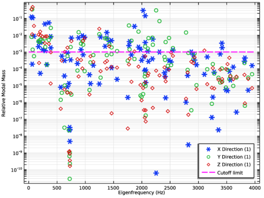
In the Settings window for Global Evaluation, type Relative Modal Mass Contribution in the Label text field.
3
Locate the Expressions section. In the table, enter the following settings:
4
Click  Evaluate.
Table
1
Go to the Table window.
2
Click Table Graph in the window toolbar.
Results
Table Graph 1
1
In the Model Builder window, under Results>1D Plot Group 2 click Table Graph 1.
2
In the Settings window for Table Graph, locate the Coloring and Style section.
3
Find the Line style subsection. From the Line list, choose None.
4
Find the Line markers subsection. From the Marker list, choose Cycle.
5
Click to expand the Legends section. Select the Show legends check box.
6
In the 1D Plot Group 2 toolbar, click  Plot.
7
Click the  y-Axis Log Scale button in the Graphics toolbar.
Modal Mass Distribution
1
In the Model Builder window, under Results click 1D Plot Group 2.
2
In the Settings window for 1D Plot Group, type Modal Mass Distribution in the Label text field.
3
Locate the Plot Settings section.
4
Select the y-axis label check box. In the associated text field, type Relative Modal Mass.
5
Locate the Legend section. From the Position list, choose Lower right.
6
In the Modal Mass Distribution toolbar, click  Plot.
Line Segments 1
1
Right-click Modal Mass Distribution and choose Line Segments.
2
In the Settings window for Line Segments, locate the x-Coordinates section.
3
4
Locate the y-Coordinates section. In the table, enter the following settings:
5
Click to expand the Coloring and Style section. From the Color list, choose Magenta.
6
Find the Line style subsection. From the Line list, choose Dashed.
7
Click to expand the Legends section. Select the Show legends check box.
8
From the Legends list, choose Manual.
9
10
Locate the Data section. From the Dataset list, choose Study: Eigenfrequency/Solution 1 (sol1).
11
From the Eigenfrequency selection list, choose First.
12
In the Modal Mass Distribution toolbar, click  Plot.
Add a filter so that the random vibration analyses can be performed using only relevant eigenmodes. This will speed up result evaluations significantly. Here, the already existing Response Spectrum node is used to obtain the structural mass. In general, you would have to add a Mass Properties node to compute the mass of the structure.
Add Study
1
In the Home toolbar, click  Add Study to open the Add Study window.
2
Go to the Add Study window.
3
Find the Studies subsection. In the Select Study tree, select Empty Study.
4
5
In the Home toolbar, click  Add Study to close the Add Study window.
Mode Filter
In the Settings window for Study, type Mode Filter in the Label text field.
Combine Solutions
1
In the Study toolbar, click  Combine Solutions.
2
In the Settings window for Combine Solutions, locate the Combine Solutions Settings section.
3
From the Solution operation list, choose Remove solutions.
4
From the Solution list, choose Study: Eigenfrequency/Solution 1 (sol1).
5
From the Exclude method list, choose Implicit.
6
In the Excluded if text field, type (comp1.rsp1.mEffLX<comp1.rsp1.mass*0.001)&&(comp1.rsp1.mEffLY<comp1.rsp1.mass*0.001)&&(comp1.rsp1.mEffLZ<comp1.rsp1.mass*0.001).
7
In the Study toolbar, click  Compute.
Add studies for a random vibration analysis. The eigenmodes are already computed, so the newly generated Study 3 can be removed.
Add Study
1
In the Study toolbar, click  Add Study to open the Add Study window.
2
Go to the Add Study window.
3
Find the Studies subsection. In the Select Study tree, select Preset Studies for Selected Physics Interfaces>Random Vibration (PSD).
4
5
In the Study toolbar, click  Add Study to close the Add Study window.
Study: ROM building
In the Settings window for Study, type Study: ROM building in the Label text field.
Step 1: Model Reduction
1
In the Model Builder window, under Study: ROM building click Step 1: Model Reduction.
2
In the Settings window for Model Reduction, locate the Model Reduction Settings section.
3
From the Training study for eigenmodes list, choose Mode Filter.
Study 3
In the Model Builder window, right-click Study 3 and choose Delete.
Add functions describing the acceleration spectrum. The logarithms are used in order to ensure a linear interpolation in a log-log space. Since the original spectrum is defined in units of g^2/Hz, it should be converted to SI units.
Global Definitions
Interpolation 1 (int1)
1
In the Home toolbar, click  Functions and choose Global>Interpolation.
2
In the Settings window for Interpolation, locate the Units section.
3
In the Function table, enter the following settings:
4
In the Argument table, enter the following settings:
5
Locate the Definition section. In the table, enter the following settings:
Since the acceleration spectrum is defined in terms of logarithms, wrap it in another function to perform the conversion.
Piecewise 1 (pw1)
1
In the Home toolbar, click  Functions and choose Global>Piecewise.
2
In the Settings window for Piecewise, type PSD in the Function name text field.
3
Locate the Definition section. In the Argument text field, type f.
4
Find the Intervals subsection. In the table, enter the following settings:
5
From the Extrapolation list, choose Specific value.
6
Locate the Units section. In the Arguments text field, type Hz.
7
In the Function text field, type m^2/s^3.
8
Click  Create Plot.
Results
Acceleration Spectrum
1
In the Settings window for 1D Plot Group, type Acceleration Spectrum in the Label text field.
2
Click the  x-Axis Log Scale button in the Graphics toolbar.
3
Click the  y-Axis Log Scale button in the Graphics toolbar.
Create the parameters (ROM controls) that are going to be used for the acceleration spectra.
Global Definitions
Global Reduced-Model Inputs 1
1
In the Model Builder window, expand the Global Definitions>Reduced-Order Modeling node, then click Global Reduced-Model Inputs 1.
2
In the Settings window for Global Reduced-Model Inputs, locate the Reduced-Model Inputs section.
3
Add the loads corresponding to the acceleration from the shaker table.
Solid Mechanics (solid)
Base Excitation 1
1
In the Model Builder window, under Component 1 (comp1)>Solid Mechanics (solid) click Base Excitation 1.
2
In the Settings window for Base Excitation, locate the Base Excitation section.
3
Specify the ab vector as
Add damping for the response analysis.
Linear Elastic Material 1
In the Model Builder window, click Linear Elastic Material 1.
Damping 1
1
In the Physics toolbar, click  Attributes and choose Damping.
2
In the Settings window for Damping, locate the Damping Settings section.
3
From the Input parameters list, choose Damping ratios.
4
In the f1 text field, type 40.
5
In the ζ1 text field, type 0.04.
6
In the f2 text field, type 1000.
7
In the ζ2 text field, type 0.04.
Make sure that the damping is not used if the eigenfrequency study is run again.
Study: Eigenfrequency
Step 1: Eigenfrequency
1
In the Model Builder window, under Study: Eigenfrequency click Step 1: Eigenfrequency.
2
In the Settings window for Eigenfrequency, locate the Physics and Variables Selection section.
3
Select the Modify model configuration for study step check box.
4
In the tree, select Component 1 (comp1)>Solid Mechanics (solid)>Linear Elastic Material 1>Damping 1.
5
Create a ROM based on the most relevant eigenmodes.
Study: ROM building
In the Home toolbar, click  Compute.
Provide random vibration spectra, and update the ROM with it.
Global Definitions
Random Vibration, X
1
In the Model Builder window, under Global Definitions>Reduced-Order Modeling click Random Vibration 1 (rvib1).
2
In the Settings window for Random Vibration, type Random Vibration, X in the Label text field.
3
Locate the Power Spectrum section. In the table, enter the following settings:
4
Locate the Output Operator Settings section. In the Lower frequency limit text field, type fL.
5
In the Upper frequency limit text field, type fU.
6
From the Integration method list, choose User defined.
7
In the Number of integration points text field, type nF.
Study: ROM building
In the Study toolbar, click  Update Solution.
Results
Random vibration plots can take a long time to generate, so it is a good idea not to replot unless explicitly requested. Also, storing the plots in the saved file can save time when reopening the model.
1
In the Model Builder window, click Results.
2
In the Settings window for Results, locate the Update of Results section.
3
Select the Only plot when requested check box.
4
Locate the Save Data in the Model section. From the Save plot data list, choose On.
RMS absolute acceleration X-excitation
1
In the Home toolbar, click  Add Plot Group and choose 3D Plot Group.
2
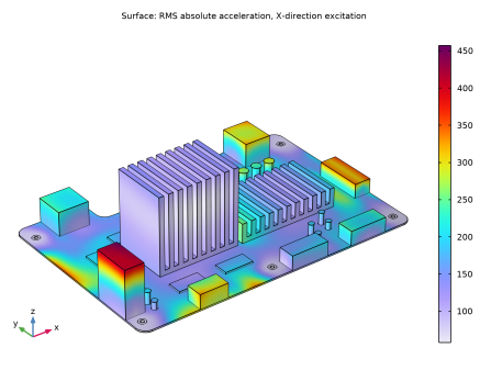
In the Settings window for 3D Plot Group, type RMS absolute acceleration X-excitation in the Label text field.
3
Locate the Data section. From the Dataset list, choose Study: ROM building/Solution 3 (sol3).
4
Click to expand the Title section. From the Title type list, choose Manual.
5
In the Title text area, type Surface: RMS absolute acceleration, X-direction excitation.
6
Click to expand the Selection section.
Surface 1
1
Right-click RMS absolute acceleration X-excitation and choose Surface.
2
In the Settings window for Surface, locate the Expression section.
3
In the Expression text field, type sqrt(rvib1.q2(solid.a_abs_rv2)).
4
Locate the Coloring and Style section. Click  Change Color Table.
5
In the Color Table dialog box, select Rainbow>Prism in the tree.
6
Switching off the refinement in the plot will give faster evaluations.
7
In the Settings window for Surface, click to expand the Quality section.
8
From the Resolution list, choose No refinement.
9
In the Model Builder window, click Surface 1.
10
In the RMS absolute acceleration X-excitation toolbar, click  Plot.
Global Definitions
Random Vibration, Y
1
In the Model Builder window, under Global Definitions>Reduced-Order Modeling right-click Random Vibration, X (rvib1) and choose Duplicate.
2
In the Settings window for Random Vibration, type Random Vibration, Y in the Label text field.
3
Locate the Power Spectrum section. In the table, enter the following settings:
Random Vibration, Z
1
Right-click Random Vibration, Y and choose Duplicate.
2
In the Settings window for Random Vibration, type Random Vibration, Z in the Label text field.
3
Locate the Power Spectrum section. In the table, enter the following settings:
Study: ROM building
In the Study toolbar, click  Update Solution.
Results
RMS absolute acceleration Y-excitation
1
Right-click RMS absolute acceleration X-excitation and choose Duplicate.
2
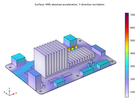
In the Settings window for 3D Plot Group, type RMS absolute acceleration Y-excitation in the Label text field.
3
Locate the Title section. In the Title text area, type Surface: RMS absolute acceleration, Y-direction excitation.
Surface 1
1
In the Model Builder window, expand the RMS absolute acceleration Y-excitation node, then click Surface 1.
2
In the Settings window for Surface, locate the Expression section.
3
In the Expression text field, type sqrt(rvib2.q2(solid.a_abs_rv2)).
4
In the RMS absolute acceleration Y-excitation toolbar, click  Plot.
RMS absolute acceleration Z-excitation
1
In the Model Builder window, right-click RMS absolute acceleration Y-excitation and choose Duplicate.
2
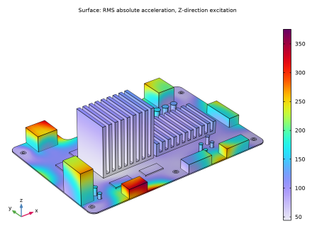
In the Settings window for 3D Plot Group, type RMS absolute acceleration Z-excitation in the Label text field.
3
Locate the Title section. In the Title text area, type Surface: RMS absolute acceleration, Z-direction excitation.
Surface 1
1
In the Model Builder window, expand the RMS absolute acceleration Z-excitation node, then click Surface 1.
2
In the Settings window for Surface, locate the Expression section.
3
In the Expression text field, type sqrt(rvib3.q2(solid.a_abs_rv2)).
4
In the RMS absolute acceleration Z-excitation toolbar, click  Plot.
After the examination of the RMS plots, select a point where the acceleration is high in all directions and study the PSD in that location.
Definitions
Average 1 (aveop1)
1
In the Definitions toolbar, click  Nonlocal Couplings and choose Average.
2
In the Settings window for Average, locate the Source Selection section.
3
From the Geometric entity level list, choose Point.
4
5
Locate the Advanced section. From the Frame list, choose Material  (X, Y, Z).
Variables 1
1
In the Model Builder window, right-click Definitions and choose Variables.
2
In the Settings window for Variables, locate the Variables section.
3
After having added new variables, the reduced-order models must be rebuilt. In this case, it would have been possible to avoid the creation of new variables, since an at3() operator could be used instead. That, however, requires that you find the coordinates of the point where you want to examine the value.
Study: ROM building
In the Home toolbar, click  Compute.
Results
Global Evaluation Sweep, X-excitation Acceleration PSD
1
In the Results toolbar, click  More Derived Values and choose Other>Global Evaluation Sweep.
Evaluate the acceleration PSD functions. In order to get values in a space fixed frame, the input PSD must be added in the excitation direction.
2
In the Settings window for Global Evaluation Sweep, type Global Evaluation Sweep, X-excitation Acceleration PSD in the Label text field.
3
Locate the Data section. From the Dataset list, choose Study: ROM building/Solution 3 (sol3).
4
Locate the Parameters section. In the table, enter the following settings:
5
Locate the Expressions section. In the table, enter the following settings:
6
Click  Evaluate.
Table
1
Go to the Table window.
2
Click Table Graph in the window toolbar.
Results
Table Graph 1
1
In the Model Builder window, under Results>1D Plot Group 7 click Table Graph 1.
2
In the Settings window for Table Graph, locate the Legends section.
3
Select the Show legends check box.
4
Click the  x-Axis Log Scale button in the Graphics toolbar.
5
Click the  y-Axis Log Scale button in the Graphics toolbar.
Absolute acceleration PSD X-excitation
1
In the Model Builder window, under Results click 1D Plot Group 7.
2
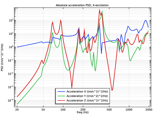
In the Settings window for 1D Plot Group, type Absolute acceleration PSD X-excitation in the Label text field.
3
Locate the Plot Settings section.
4
Select the y-axis label check box. In the associated text field, type PSD ((m/s^2)^2/Hz).
5
Locate the Legend section. From the Position list, choose Lower middle.
6
Click to expand the Title section. From the Title type list, choose Manual.
7
In the Title text area, type Absolute acceleration PSD, X-excitation.
8
In the Absolute acceleration PSD X-excitation toolbar, click  Plot.
Global Evaluation Sweep, Y-excitation Acceleration PSD
1
In the Model Builder window, right-click Global Evaluation Sweep, X-excitation Acceleration PSD and choose Duplicate.
2
In the Settings window for Global Evaluation Sweep, type Global Evaluation Sweep, Y-excitation Acceleration PSD in the Label text field.
3
Locate the Expressions section. In the table, enter the following settings:
4
Clicknext to  Evaluate, then choose New Table.
Absolute acceleration PSD Y-excitation
1
In the Model Builder window, right-click Absolute acceleration PSD X-excitation and choose Duplicate.
2
In the Model Builder window, click Absolute acceleration PSD X-excitation 1.
3
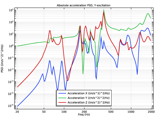
In the Settings window for 1D Plot Group, type Absolute acceleration PSD Y-excitation in the Label text field.
4
Locate the Title section. In the Title text area, type Absolute acceleration PSD, Y-excitation.
Table Graph 1
1
In the Model Builder window, click Table Graph 1.
2
In the Settings window for Table Graph, locate the Data section.
3
From the Table list, choose Table 4.
4
In the Absolute acceleration PSD Y-excitation toolbar, click  Plot.
Global Evaluation Sweep, Z-excitation Acceleration PSD
1
In the Model Builder window, right-click Global Evaluation Sweep, Y-excitation Acceleration PSD and choose Duplicate.
2
In the Settings window for Global Evaluation Sweep, type Global Evaluation Sweep, Z-excitation Acceleration PSD in the Label text field.
3
Locate the Expressions section. In the table, enter the following settings:
4
Clicknext to  Evaluate, then choose New Table.
Absolute acceleration PSD Z-excitation
1
In the Model Builder window, right-click Absolute acceleration PSD Y-excitation and choose Duplicate.
2
In the Model Builder window, click Absolute acceleration PSD Y-excitation 1.
3
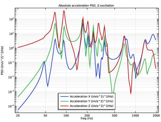
In the Settings window for 1D Plot Group, type Absolute acceleration PSD Z-excitation in the Label text field.
4
Locate the Title section. In the Title text area, type Absolute acceleration PSD, Z-excitation.
Table Graph 1
1
In the Model Builder window, click Table Graph 1.
2
In the Settings window for Table Graph, locate the Data section.
3
From the Table list, choose Table 5.
4
In the Absolute acceleration PSD Z-excitation toolbar, click  Plot.
Check the bolt forces.
Bolt Forces X-excitation
1
In the Results toolbar, click  Global Evaluation.
2
In the Settings window for Global Evaluation, type Bolt Forces X-excitation in the Label text field.
3
Locate the Data section. From the Dataset list, choose Study: ROM building/Solution 3 (sol3).
4
Locate the Expressions section. Click  Load from File.
5
6
Click  Evaluate.
Bolt Forces Y-excitation
1
In the Results toolbar, click  Global Evaluation.
2
In the Settings window for Global Evaluation, type Bolt Forces Y-excitation in the Label text field.
3
Locate the Data section. From the Dataset list, choose Study: ROM building/Solution 3 (sol3).
4
Locate the Expressions section. Click  Load from File.
5
6
Click  Evaluate.
Bolt Forces Z-excitation
1
In the Results toolbar, click  Global Evaluation.
2
In the Settings window for Global Evaluation, type Bolt Forces Z-excitation in the Label text field.
3
Locate the Data section. From the Dataset list, choose Study: ROM building/Solution 3 (sol3).
4
Locate the Expressions section. Click  Load from File.
5
6
Click  Evaluate.