|
|
|
|
1
|
|
2
|
|
3
|
|
4
|
Click
|
|
5
|
|
6
|
Click
|
|
1
|
|
2
|
|
3
|
|
1
|
|
2
|
|
3
|
Click
|
|
4
|
Browse to the model’s Application Libraries folder and double-click the file main_bearing_cap_geom.mphbin.
|
|
5
|
Click
|
|
1
|
|
2
|
|
3
|
|
4
|
On the object imp1(1), select Boundary 4 only.
|
|
1
|
|
2
|
|
3
|
|
4
|
|
1
|
In the Model Builder window, under Component 1 (comp1)>Geometry 1 click Hex Bolt, With Drill 1 (pi1).
|
|
2
|
|
3
|
|
4
|
Locate the Position and Orientation of Output section. Find the Coordinate system in part subsection. From the Work plane in part list, choose Head inner plane (wp1).
|
|
5
|
Find the Coordinate system to match subsection. From the Work plane list, choose Work Plane 1 (wp1).
|
|
6
|
|
7
|
|
8
|
Click OK.
|
|
9
|
|
11
|
|
12
|
|
1
|
|
2
|
|
3
|
Locate the Position and Orientation of Output section. Find the Displacement subsection. In the xw text field, type 55.
|
|
1
|
|
2
|
Select the object imp1(2) only.
|
|
3
|
|
4
|
|
5
|
|
6
|
|
1
|
|
2
|
|
3
|
|
4
|
|
5
|
|
1
|
|
2
|
|
4
|
|
1
|
|
2
|
|
3
|
|
4
|
|
5
|
|
6
|
Click OK.
|
|
1
|
|
2
|
In the Settings window for Adjacent, type Stress Area Reduced Domains Domains in the Label text field.
|
|
3
|
|
4
|
|
5
|
|
6
|
|
7
|
Click OK.
|
|
1
|
|
2
|
|
3
|
|
4
|
|
5
|
|
6
|
|
7
|
Click OK.
|
|
1
|
|
2
|
|
3
|
|
4
|
|
5
|
|
1
|
In the Model Builder window, under Component 1 (comp1)>Materials right-click Structural steel (mat1) and choose Duplicate.
|
|
2
|
|
3
|
Locate the Geometric Entity Selection section. From the Selection list, choose Stress Area Reduced Domains Domains.
|
|
4
|
|
1
|
In the Model Builder window, under Component 1 (comp1)>Definitions click Identity Boundary Pair 1 (ap1).
|
|
2
|
|
3
|
|
4
|
|
5
|
|
6
|
|
7
|
Click OK.
|
|
8
|
|
9
|
|
10
|
|
11
|
Click OK.
|
|
12
|
|
13
|
|
14
|
|
1
|
|
2
|
|
3
|
|
4
|
|
5
|
|
1
|
|
2
|
|
3
|
|
4
|
|
5
|
|
1
|
|
1
|
|
2
|
|
3
|
|
4
|
|
1
|
|
2
|
|
3
|
|
1
|
|
2
|
|
3
|
|
1
|
|
2
|
|
3
|
|
4
|
|
5
|
Click OK.
|
|
6
|
|
7
|
|
8
|
|
9
|
|
10
|
|
11
|
|
1
|
|
3
|
|
4
|
|
1
|
|
2
|
|
3
|
|
4
|
|
1
|
|
2
|
|
3
|
|
4
|
|
5
|
|
6
|
|
7
|
|
1
|
|
2
|
|
3
|
|
4
|
|
5
|
|
6
|
|
7
|
|
1
|
|
2
|
|
3
|
|
4
|
|
5
|
|
6
|
|
7
|
|
8
|
|
1
|
|
2
|
|
3
|
|
4
|
Click
|
|
1
|
|
2
|
|
3
|
In the Model Builder window, expand the Study 1>Solver Configurations>Solution 1 (sol1)>Stationary Solver 1>Segregated 1 node, then click Solid Mechanics.
|
|
4
|
|
5
|
|
6
|
Click
|
|
1
|
|
2
|
|
3
|
|
1
|
|
2
|
|
3
|
|
4
|
|
1
|
|
2
|
|
1
|
|
2
|
|
3
|
|
4
|
|
5
|
|
6
|
|
1
|
|
3
|
|
1
|
|
2
|
|
1
|
|
2
|
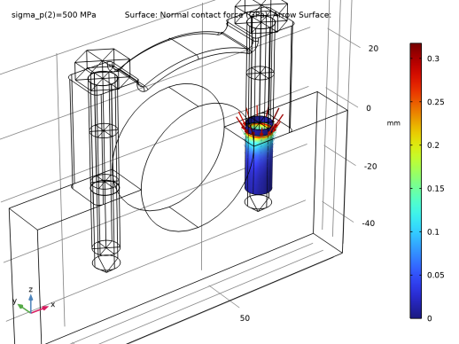
In the Settings window for Surface, click Replace Expression in the upper-right corner of the Expression section. From the menu, choose Component 1 (comp1)>Solid Mechanics>Bolts>Bolt thread contact>solid.Fn_up - Normal contact force - N/m².
|
|
3
|
|
1
|
|
2
|
|
3
|
|
4
|
|
5
|
|
6
|
|
7
|
|
8
|
|
1
|
|
2
|
|
3
|
|
4
|
|
5
|
|
1
|
|
2
|
|
3
|
|
4
|
|
1
|
|
2
|
In the Settings window for 2D Plot Group, type Contact Pressure Between Caps in the Label text field.
|
|
1
|
|
2
|
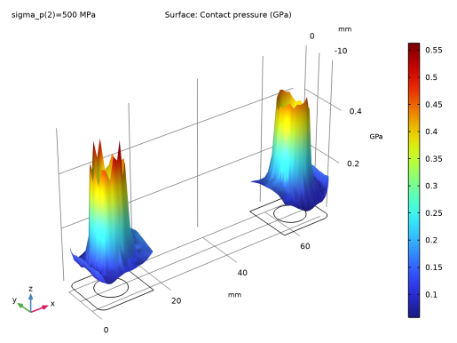
In the Settings window for Surface, click Replace Expression in the upper-right corner of the Expression section. From the menu, choose Component 1 (comp1)>Solid Mechanics>Contact>solid.Tn - Contact pressure - N/m².
|
|
3
|
|
1
|
|
2
|