|
|
|
|
3
|

|
1
|
|
2
|
|
3
|
Click Add.
|
|
4
|
Click
|
|
5
|
|
6
|
Click
|
|
1
|
|
2
|
|
1
|
In the Model Builder window, right-click Global Definitions and choose Load and Constraint Groups>Load Group.
|
|
2
|
|
3
|
|
1
|
|
2
|
|
3
|
|
1
|
|
2
|
|
3
|
|
1
|
|
2
|
On the object pol1, select Edge 1 only.
|
|
3
|
|
5
|
|
1
|
In the Model Builder window, under Component 1 (comp1) right-click Materials and choose Blank Material.
|
|
2
|
|
1
|
|
2
|
|
3
|
|
4
|
|
5
|
In the Show More Options dialog box, in the tree, select the check box for the node Physics>Advanced Physics Options.
|
|
6
|
Click OK.
|
|
7
|
|
8
|
|
1
|
|
3
|
|
4
|
|
5
|
|
6
|
|
7
|
|
1
|
|
2
|
|
3
|
|
4
|
|
5
|
|
6
|
|
1
|
|
2
|
|
4
|
|
5
|
|
1
|
|
2
|
|
4
|
|
1
|
|
2
|
|
3
|
Specify the u vector as
|
|
1
|
|
2
|
|
3
|
|
1
|
|
2
|
|
3
|
Click the Custom button.
|
|
4
|
Locate the Element Size Parameters section. In the Maximum element size text field, type L_cable/60.
|
|
5
|
|
6
|
|
1
|
|
2
|
|
3
|
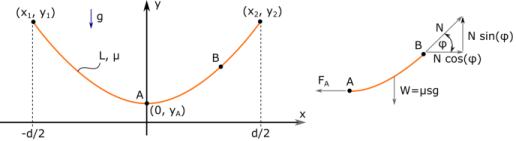
Locate the Definition section. In the Expression text field, type a*(cosh(X/a) - cosh(0.5*d_support/a)).
|
|
4
|
|
5
|
|
1
|
|
2
|
|
3
|
|
4
|
|
5
|
|
1
|
In the Model Builder window, under Component 2 (comp2)>Global ODEs and DAEs (ge) click Global Equations 1.
|
|
2
|
|
4
|
|
5
|
|
6
|
Click
|
|
7
|
|
8
|
Click OK.
|
|
9
|
|
10
|
|
11
|
|
12
|
Click OK.
|
|
1
|
|
2
|
|
3
|
|
4
|
Click
|
|
1
|
|
2
|
|
3
|
|
4
|
|
5
|
In the Model Builder window, expand the Study 1>Solver Configurations>Solution 1 (sol1)>Stationary Solver 1 node, then click Fully Coupled 1.
|
|
6
|
|
7
|
|
8
|
|
1
|
|
2
|
|
3
|
|
1
|
|
2
|
|
3
|
|
4
|
|
5
|
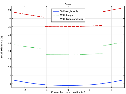
Select the x-axis label check box. In the associated text field, type Current horizontal position (m).
|
|
6
|
|
7
|
|
8
|
|
1
|
|
2
|
|
3
|
|
4
|
|
5
|
|
6
|
|
7
|
|
8
|
|
10
|
Click to expand the Coloring and Style section. Find the Line style subsection. From the Line list, choose Cycle.
|
|
11
|
|
1
|
|
2
|
|
3
|
|
4
|
|
1
|
|
2
|
|
3
|
|
4
|
|
5
|
|
6
|
Locate the Legends section. In the table, enter the following settings:
|
|
7
|
|
1
|
|
2
|
|
3
|
|
4
|
|
5
|
Select the x-axis label check box. In the associated text field, type Current horizontal position (m).
|
|
6
|
|
1
|
|
2
|
|
3
|
|
4
|
|
5
|
|
6
|
|
7
|
Locate the Coloring and Style section. Find the Line style subsection. From the Line list, choose Cycle.
|
|
8
|
|
9
|
|
10
|
|
11
|
|
1
|
|
2
|
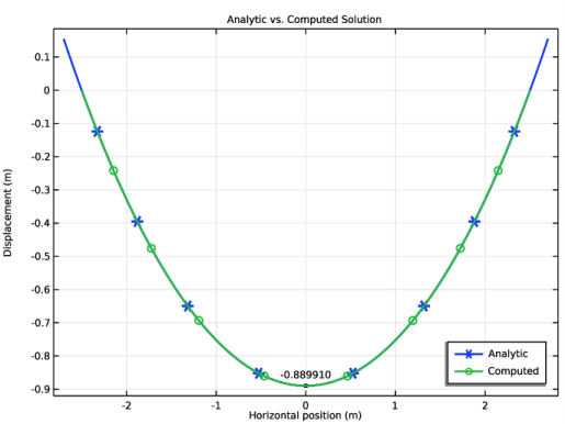
In the Settings window for 1D Plot Group, type Analytic vs. Computed Solution in the Label text field.
|
|
3
|
|
4
|
|
5
|
|
6
|
|
7
|
|
8
|
|
1
|
|
2
|
|
3
|
|
4
|
Locate the y-Axis Data section. In the Expression text field, type y_catenary(X, comp2.a, d_support).
|
|
5
|
|
6
|
|
7
|
|
8
|
|
9
|
|
10
|
|
11
|
|
1
|
|
2
|
|
3
|
|
4
|
|
1
|
|
2
|
|
3
|
|
4
|
|
5
|
Locate the Legends section. In the table, enter the following settings:
|
|
6
|