PDF

Modeling of Pretensioned Bolts
Introduction
In many structures, joined parts are clamped by bolts. In order to obtain a good clamping effect, the bolts are tightened so that the axial stresses are high. In an analysis, a correct state of the prestressed structure is often essential when evaluating the effect of service loads. For example, friction forces between joined parts may be crucial for the load carrying capacity. Also, if the effect of the pretension is ignored, the change in bolt forces due to service loads may be overestimated by one order of magnitude.
In most cases, the tensioning order of the bolts has little effect. However, if there are significant nonlinear phenomena, such as plasticity or frictional sliding, the sequence may have to be taken into consideration in the analysis.
In this example, different approaches for modeling pretensioned bolts are explored. The geometry does not show any realistic structure, as the focus is entirely on bolt modeling.
Model Definition
Two steel plates, 150 mm-by-100 mm, are joined using five M10 bolts. The upper plate has a thickness of 10 mm and the lower plate has a thickness of 20 mm. There is an internal cavity formed by matching imprints in the two plates. The geometry is shown in Figure 1.
Two of the bolts are modeled with solid elements, and three by using beam elements. The connections to the plates are created by using different approximations.
Figure 1: The geometry of the component, and the bolt numbering.
Details about how the bolts are modeled are given in Table 1.
The final prestress force in the bolts is set to P = 50 kN. However, not all bolts are tightened to the full prestress force simultaneously. Rather, the bolts are tightened one by one, with the three first bolts tightened only to 70% of the full value during the first cycle. In all, there are eight steps in the tightening cycle, as summarized in Table 2.
Between the two plates, as well as under the head of Bolt 4, there are contact conditions. The coefficient of friction is assumed to be 0.15 everywhere.
The service load is an internal pressure with a maximum value of 4 MPa.
Results and Discussion
Table 3 summarizes the bolt forces in the different steps of the pretensioning sequence. As can be seen, the variation of the bolt forces from their prescribed values is very small in this case. Typically, the force in the already tightened bolts drops somewhat due to the compression from the neighboring bolts.
Note that the inactive bolts actually have been assigned a very small force; 1% of the final force. This will make the analysis run much faster than if the bolts were without force. The reason is that the contact problem has a very slow convergence rate when two boundaries are barely touching. There are other possible approaches, for example including gravity in the analysis, so that the upper plate rests slightly on the lower plate.
Figure 2 shows stresses in the bolts as well as the contact pressure between the upper and the lower block.
Figure 2: Stresses in the bolts and contact pressure between the plates after the tightening sequence.
All bolts have the same stress at the cross section where the bolt prestress is applied. In the bolts modeled with beam elements, the stress is exact and uniform all through the length, whereas when the bolts are modeled as solids, this is only true in an average sense. The detailed stress field is affected by stress concentrations.
The distribution of the contact pressure differs between the through bolts and the bolts that end in an internal thread. In the latter case, the pressure is higher close to the holes, since the path of the force is shorter. Note also that there is a significant contact pressure only in a circle within a diameter of two to three times the hole size. This is why, in practice, gaskets are needed to avoid leakage.
In Figure 3 shows the transverse (Z direction) stress in the top and bottom blocks. As can be seen, the general picture is the same, irrespective of whether the bolt is modeled using beams or solid elements. The details of the stress field at the threads is more sensitive. When modeling with beams, it is important to use a suitable effective bolt length, as well as a suitable coupling length inside the thread.
Figure 3: Stress in the Z direction at the bolt holes after the tightening sequence.
In Figure 4 to Figure 6, the bolt stress and the contact pressures are shown for three different levels of the internal pressure in the cavity. There is a significant redistribution of the contact pressure at higher load levels, which indicates that the joints are no longer operating as intended.
Figure 4: Stresses in the bolts and contact pressure between the plates after applying 20% of the service load.
Figure 5: Stresses in the bolts and contact pressure between the plates after applying 50% of the service load.
Figure 6: Stresses in the bolts and contact pressure between the plates after applying 100% of the service load.
Application Library path: Structural_Mechanics_Module/Tutorials/bolt_pretension_tutorial
Modeling Instructions
From the File menu, choose New.
New
In the New window, click  Model Wizard.
Model Wizard
1
In the Model Wizard window, click  3D.
2
In the Select Physics tree, select Structural Mechanics>Solid Mechanics (solid) and Structural Mechanics>Beam (beam).
3
Click Add.
4
Click  Study.
5
In the Select Study tree, select Preset Studies for Selected Physics Interfaces>Bolt Pretension.
6
Global Definitions
Parameters 1
1
In the Model Builder window, under Global Definitions click Parameters 1.
2
In the Settings window for Parameters, locate the Parameters section.
3
Click  Load from File.
4
Geometry 1
1
In the Model Builder window, under Component 1 (comp1) click Geometry 1.
2
In the Settings window for Geometry, locate the Units section.
3
From the Length unit list, choose mm.
Form Union (fin)
1
In the Model Builder window, expand the Geometry 1 node, then click Form Union (fin).
2
In the Settings window for Form Union/Assembly, locate the Form Union/Assembly section.
3
From the Action list, choose Form an assembly.
Block: Bottom
1
In the Geometry toolbar, click  Block.
2
In the Settings window for Block, type Block: Bottom in the Label text field.
3
Locate the Size and Shape section. In the Width text field, type plateLen.
4
In the Depth text field, type plateWidth.
5
In the Height text field, type thicLow.
6
Click  Build Selected.
Block: Top
1
Right-click Block: Bottom and choose Duplicate.
2
In the Settings window for Block, type Block: Top in the Label text field.
3
Locate the Position section. In the z text field, type thicLow.
4
Locate the Size and Shape section. In the Height text field, type thicUp.
5
Click  Build Selected.
Block: Cavity
1
In the Geometry toolbar, click  Block.
2
In the Settings window for Block, type Block: Cavity in the Label text field.
3
Click the  Transparency button in the Graphics toolbar.
4
Locate the Size and Shape section. In the Width text field, type plateLen/2.
5
In the Depth text field, type plateWidth/2.
6
In the Height text field, type (thicUp+thicLow)/2.
7
Locate the Position section. In the x text field, type plateLen/4.
8
In the y text field, type plateWidth/4.
9
In the z text field, type (thicUp+thicLow)/4.
Cylinder: Bolt Hole
1
In the Geometry toolbar, click  Cylinder.
2
In the Settings window for Cylinder, type Cylinder: Bolt Hole in the Label text field.
3
Locate the Size and Shape section. In the Radius text field, type holeDia/2.
4
In the Height text field, type thicLow+thicUp+2[mm].
5
Locate the Position section. In the x text field, type 20.
6
In the y text field, type 20.
7
In the z text field, type -1.
8
Click  Build Selected.
Array: Bolt Holes
1
In the Geometry toolbar, click  Transforms and choose Array.
2
In the Settings window for Array, type Array: Bolt Holes in the Label text field.
3
4
Locate the Size section. In the x size text field, type 3.
5
Locate the Displacement section. In the x text field, type boltSpacing.
6
Click  Build Selected.
Part Libraries
1
In the Geometry toolbar, click  Parts and choose Part Libraries.
2
In the Part Libraries window, select Structural Mechanics Module>Bolts>hex_bolt_no_thread in the tree.
3
Click  Add to Geometry.
Geometry 1
Hex Bolt, No Thread 1 (pi1)
1
In the Model Builder window, under Component 1 (comp1)>Geometry 1 click Hex Bolt, No Thread 1 (pi1).
2
In the Settings window for Part Instance, locate the Input Parameters section.
3
4
Locate the Position and Orientation of Output section. Find the Displacement subsection. In the xw text field, type 20.
5
In the yw text field, type 20.
6
In the zw text field, type -10.
7
Click  Build Selected.
8
Click to expand the Boundary Selections section. In the table, enter the following settings:
9
Click to expand the Domain Selections section. In the table, enter the following settings:
10
11
Click New Cumulative Selection.
12
In the New Cumulative Selection dialog box, type Bolts and Nuts in the Name text field.
13
Part Libraries
1
In the Geometry toolbar, click  Parts and choose Part Libraries.
2
In the Model Builder window, click Geometry 1.
3
In the Part Libraries window, select Structural Mechanics Module>Bolts>hex_nut in the tree.
4
Click  Add to Geometry.
Geometry 1
Hexagonal Nut 1 (pi2)
1
In the Model Builder window, under Component 1 (comp1)>Geometry 1 click Hexagonal Nut 1 (pi2).
2
In the Settings window for Part Instance, locate the Input Parameters section.
3
4
Locate the Position and Orientation of Output section. Find the Displacement subsection. In the xw text field, type 20.
5
In the yw text field, type 20.
6
In the zw text field, type -6.
7
Click  Build Selected.
8
Locate the Domain Selections section. In the table, enter the following settings:
Part Libraries
1
In the Geometry toolbar, click  Parts and choose Part Libraries.
2
In the Model Builder window, click Geometry 1.
3
In the Part Libraries window, select Structural Mechanics Module>Bolts>simple_bolt_drill in the tree.
4
Click  Add to Geometry.
Geometry 1
Simple Bolt, With Drill 1 (pi3)
1
In the Model Builder window, under Component 1 (comp1)>Geometry 1 click Simple Bolt, With Drill 1 (pi3).
2
In the Settings window for Part Instance, locate the Input Parameters section.
3
4
Locate the Position and Orientation of Output section. Find the Displacement subsection. In the xw text field, type 20.
5
In the yw text field, type plateWidth-20.
6
In the zw text field, type thicLow-threadDepth+(boltDia-1)/(2*tan(50[deg])).
7
Locate the Boundary Selections section. In the table, enter the following settings:
8
Locate the Domain Selections section. In the table, enter the following settings:
9
Click  Build All Objects.
Copy: Drill
1
In the Geometry toolbar, click  Transforms and choose Copy.
2
In the Settings window for Copy, type Copy: Drill in the Label text field.
3
Select the object pi3(2) only.
4
Locate the Displacement section. In the x text field, type 2*boltSpacing.
5
Click  Build Selected.
Difference: Bolt Holes and Cavity, Upper
1
In the Geometry toolbar, click  Booleans and Partitions and choose Difference.
2
In the Settings window for Difference, type Difference: Bolt Holes and Cavity, Upper in the Label text field.
3
4
Locate the Difference section. Select the Keep objects to subtract check box.
5
Find the Objects to subtract subsection. Click to select the  Activate Selection toggle button.
6
Select the objects arr1(1,1,1), arr1(2,1,1), arr1(3,1,1), blk3, copy1, and pi3(2) only.
7
Click  Build Selected.
Difference: Bolt Holes and Cavity, Lower
1
Right-click Difference: Bolt Holes and Cavity, Upper and choose Duplicate.
2
In the Settings window for Difference, type Difference: Bolt Holes and Cavity, Lower in the Label text field.
3
Locate the Difference section. Find the Objects to add subsection. Click to select the  Activate Selection toggle button.
4
5
Clear the Keep objects to subtract check box.
6
Click  Build Selected.
7
In the Geometry toolbar, click  Build All.
Work Plane 1 (wp1)
1
In the Geometry toolbar, click  Work Plane.
2
In the Settings window for Work Plane, locate the Plane Definition section.
3
From the Offset type list, choose Through vertex.
4
Find the Offset vertex subsection. Click to select the  Activate Selection toggle button.
5
On the object dif1, select Point 2 only.
Work Plane 1 (wp1)>Plane Geometry
In the Model Builder window, click Plane Geometry.
Circle: Imprint for Bolt Head
1
In the Work Plane toolbar, click  Circle.
2
In the Settings window for Circle, type Circle: Imprint for Bolt Head in the Label text field.
3
Locate the Object Type section. From the Type list, choose Curve.
4
Locate the Size and Shape section. In the Radius text field, type headDia/2.
5
Locate the Position section. In the xw text field, type 20+boltSpacing.
6
In the yw text field, type 20.
7
Click  Build Selected.
Copy: Imprints for Bolt Heads
1
In the Work Plane toolbar, click  Transforms and choose Copy.
2
In the Settings window for Copy, type Copy: Imprints for Bolt Heads in the Label text field.
3
4
Locate the Displacement section. In the xw text field, type boltSpacing.
5
Click  Build Selected.
Union: Imprints for Bolt Heads
1
In the Model Builder window, right-click Geometry 1 and choose Booleans and Partitions>Union.
2
In the Settings window for Union, type Union: Imprints for Bolt Heads in the Label text field.
3
Select the objects dif1 and wp1 only.
4
Click  Build All Objects.
Polygon: Bolt 2 Beam
1
In the Geometry toolbar, click  More Primitives and choose Polygon.
2
In the Settings window for Polygon, type Polygon: Bolt 2 Beam in the Label text field.
3
Locate the Coordinates section. In the table, enter the following settings:
4
Locate the Selections of Resulting Entities section. Find the Cumulative selection subsection. Click New.
5
In the New Cumulative Selection dialog box, type Beams in the Name text field.
6
Copy: Bolt 3 Beam
1
In the Geometry toolbar, click  Transforms and choose Copy.
2
In the Settings window for Copy, type Copy: Bolt 3 Beam in the Label text field.
3
4
Locate the Displacement section. In the x text field, type boltSpacing.
5
Locate the Selections of Resulting Entities section. Find the Cumulative selection subsection. From the Contribute to list, choose Bolts and Nuts.
6
Click  Build Selected.
Polygon: Bolt 5 Beam
1
In the Geometry toolbar, click  More Primitives and choose Polygon.
2
In the Settings window for Polygon, type Polygon: Bolt 5 Beam in the Label text field.
3
Locate the Coordinates section. In the table, enter the following settings:
4
Locate the Selections of Resulting Entities section. Find the Cumulative selection subsection. From the Contribute to list, choose Beams.
5
Click  Build Selected.
Take a look at the detailed bolt geometries.
6
In the Graphics window toolbar, clicknext to  Clipping, then choose Add Clip Plane.
Definitions
In the Model Builder window, expand the Component 1 (comp1)>Definitions node.
Clip Plane 1
1
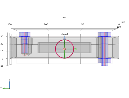
In the Model Builder window, expand the Component 1 (comp1)>Definitions>View 1 node, then click Clip Plane 1.
2
In the Settings window for Clip Plane, locate the Position section.
3
Find the Definition subsection. In the x text field, type 20.01.
4
Select the objects pi1, pi2, and pi3(1) only.
5
Click the  Go to YZ View button in the Graphics toolbar.
6
Click the  Go to YZ View button in the Graphics toolbar.
7
Click the  Go to YZ View button in the Graphics toolbar.
8
In the Graphics window toolbar, clicknext to  Clipping Active, then choose Show Frames.
9
Click the  Zoom Extents button in the Graphics toolbar.
10
In the Graphics window toolbar, clicknext to  Clipping, then choose Delete Plane1.
Root
Click the  Go to Default View button in the Graphics toolbar.
Beam (beam)
1
In the Model Builder window, under Component 1 (comp1) click Beam (beam).
2
In the Settings window for Beam, locate the Edge Selection section.
3
From the Selection list, choose Beams.
Cross Section M10
1
In the Model Builder window, under Component 1 (comp1)>Beam (beam) click Cross-Section Data 1.
2
In the Settings window for Cross-Section Data, type Cross Section M10 in the Label text field.
3
Locate the Cross-Section Definition section. From the list, choose Common sections.
4
From the Section type list, choose Circular.
5
In the do text field, type boltDia.
Section Orientation 1
1
In the Model Builder window, click Section Orientation 1.
2
In the Settings window for Section Orientation, locate the Section Orientation section.
3
From the Orientation method list, choose Orientation vector.
4
Specify the V vector as
Add Material
1
In the Home toolbar, click  Add Material to open the Add Material window.
2
Go to the Add Material window.
3
In the tree, select Built-in>Structural steel.
4
Right-click and choose Add to Global Materials.
5
In the Home toolbar, click  Add Material to close the Add Material window.
Materials
Material Link 1 (matlnk1)
In the Model Builder window, under Component 1 (comp1) right-click Materials and choose More Materials>Material Link.
Material Link 2 (matlnk2)
1
Right-click Materials and choose More Materials>Material Link.
2
In the Settings window for Material Link, locate the Geometric Entity Selection section.
3
From the Geometric entity level list, choose Edge.
4
From the Selection list, choose Beams.
Bolt 2 is connected using rigid connectors. Create the Solid Mechanics part.
Solid Mechanics (solid)
In the Model Builder window, under Component 1 (comp1) click Solid Mechanics (solid).
RC Bolt 2, Head
1
In the Physics toolbar, click  Boundaries and choose Rigid Connector.
2
In the Settings window for Rigid Connector, type RC Bolt 2, Head in the Label text field.
3
RC Bolt 2, Nut
1
In the Physics toolbar, click  Edges and choose Rigid Connector.
2
In the Settings window for Rigid Connector, type RC Bolt 2, Nut in the Label text field.
3
In the continuity conditions, connections will be established between mismatching meshes. It is often more efficient to use a Nitsche formulation than a large number of coupled pointwise constraints.
Continuity 1
1
In the Model Builder window, click Continuity 1.
2
In the Settings window for Continuity, locate the Method section.
3
Beam (beam)
Add the Beam side of the rigid connectors. In order to couple the rigid connectors between the physics interfaces, Advanced Physics Options must be enabled.
In the Model Builder window, under Component 1 (comp1) click Beam (beam).
RC Bolt 2, Head
1
In the Physics toolbar, click  Points and choose Rigid Connector.
2
Click the  Show More Options button in the Model Builder toolbar.
3
In the Show More Options dialog box, select Physics>Advanced Physics Options in the tree.
4
In the tree, select the check box for the node Physics>Advanced Physics Options.
5
6
In the Settings window for Rigid Connector, type RC Bolt 2, Head in the Label text field.
7
8
Click to expand the Advanced section. From the Connect to list, choose RC Bolt 2, Head (solid).
RC Bolt 2, Nut
1
In the Physics toolbar, click  Points and choose Rigid Connector.
2
In the Settings window for Rigid Connector, type RC Bolt 2, Nut in the Label text field.
3
4
Locate the Advanced section. From the Connect to list, choose RC Bolt 2, Nut (solid).
Multiphysics
SBC, Bolt 3, Head
1
In the Physics toolbar, click  Multiphysics Couplings and choose Global>Solid-Beam Connection.
2
In the Settings window for Solid-Beam Connection, type SBC, Bolt 3, Head in the Label text field.
3
Locate the Connection Settings section. Select the Manual control of selections check box.
4
5
Locate the Point Selection, Beam section. Click to select the  Activate Selection toggle button.
6
SBC, Bolt 3, Nut
1
In the Physics toolbar, click  Multiphysics Couplings and choose Global>Solid-Beam Connection.
2
In the Settings window for Solid-Beam Connection, type SBC, Bolt 3, Nut in the Label text field.
3
Locate the Connection Settings section. From the Connection type list, choose Solid edges to beam points.
4
Locate the Edge Selection, Solid section. Click to select the  Activate Selection toggle button.
5
6
Locate the Point Selection, Beam section. Click to select the  Activate Selection toggle button.
7
SBC, Bolt 5, Head
1
In the Physics toolbar, click  Multiphysics Couplings and choose Global>Solid-Beam Connection.
2
In the Settings window for Solid-Beam Connection, type SBC, Bolt 5, Head in the Label text field.
3
Locate the Connection Settings section. Select the Manual control of selections check box.
4
5
Locate the Point Selection, Beam section. Click to select the  Activate Selection toggle button.
6
7
Locate the Connection Settings section. From the Connected region list, choose Distance (manual).
8
In the rc text field, type headDia/2.
SBC, Bolt 5, Thread
1
In the Physics toolbar, click  Multiphysics Couplings and choose Global>Solid-Beam Connection.
2
In the Settings window for Solid-Beam Connection, type SBC, Bolt 5, Thread in the Label text field.
3
Locate the Connection Settings section. Select the Manual control of selections check box.
4
5
Locate the Point Selection, Beam section. Click to select the  Activate Selection toggle button.
6
7
Locate the Connection Settings section. From the Connected region list, choose Connection criterion.
8
In the text field, type Z>thicLow-boltDia/2.
Global Definitions
Create functions returning the prestress values and the times when they are changed. Using such functions makes the input in each Bolt Selection node more readable.
Analytic 1 (an1)
1
In the Home toolbar, click  Functions and choose Global>Analytic.
2
In the Settings window for Analytic, type forceValue in the Function name text field.
3
Locate the Definition section. In the Arguments text field, type active,full,time.
4
In the Expression text field, type if(time<active,0.01,if(time<full,0.7,1)).
5
Locate the Units section. In the Function text field, type 1.
6
Analytic 2 (forceValue2)
1
Right-click Analytic 1 (forceValue) and choose Duplicate.
2
In the Settings window for Analytic, type setPre in the Function name text field.
3
Locate the Definition section. In the Expression text field, type time==1 || abs(time-active)<0.001 || abs(time-full)<0.001.
Solid Mechanics (solid)
In the Model Builder window, under Component 1 (comp1) click Solid Mechanics (solid).
Bolt Pretension 1
1
In the Physics toolbar, click  Global and choose Bolt Pretension.
2
In the Settings window for Bolt Pretension, locate the Bolt Pretension section.
3
In the Fp text field, type boltForce.
4
Select the Compute tightening torque check box.
5
In the l text field, type 1.5[mm].
6
From the Bolt head type list, choose Hexagonal.
Bolt Selection 1
1
In the Model Builder window, expand the Bolt Pretension 1 node, then click Bolt Selection 1.
2
In the Settings window for Bolt Selection, locate the Boundary Selection section.
3
From the Selection list, choose Pretension cut (Hex Bolt, No Thread 1).
4
Locate the Bolt Pretension section. Select the Sequential tightening check box.
5
From the Pretension type list, choose Pretension force.
6
In the Fp text field, type boltForce*forceValue(1,6,par).
7
In the Pretensioning expression text field, type setPre(1,6,par).
Bolt Pretension 1
In the Model Builder window, click Bolt Pretension 1.
Bolt Selection 2
1
In the Physics toolbar, click  Attributes and choose Bolt Selection.
2
In the Settings window for Bolt Selection, locate the Bolt Label section.
3
4
Locate the Boundary Selection section. From the Selection list, choose Pretension cut (Simple Bolt, With Drill 1).
5
Locate the Bolt Pretension section. Select the Sequential tightening check box.
6
From the Pretension type list, choose Pretension force.
7
In the Fp text field, type boltForce*forceValue(4,4,par).
8
In the Pretensioning expression text field, type setPre(4,4,par).
Beam (beam)
In the Model Builder window, under Component 1 (comp1) click Beam (beam).
Bolt Pretension 1
1
In the Physics toolbar, click  Global and choose Bolt Pretension.
2
In the Settings window for Bolt Pretension, locate the Bolt Pretension section.
3
In the Fp text field, type boltForce.
Bolt Selection 1
1
In the Model Builder window, expand the Bolt Pretension 1 node, then click Bolt Selection 1.
2
In the Settings window for Bolt Selection, locate the Bolt Label section.
3
4
5
Locate the Bolt Pretension section. Select the Sequential tightening check box.
6
From the Pretension type list, choose Pretension force.
7
In the Fp text field, type boltForce*forceValue(2,7,par).
8
In the Pretensioning expression text field, type setPre(2,7,par).
Bolt Selection 2
1
Right-click Component 1 (comp1)>Beam (beam)>Bolt Pretension 1>Bolt Selection 1 and choose Duplicate.
2
In the Settings window for Bolt Selection, locate the Bolt Label section.
3
4
Locate the Point Selection section. Click  Clear Selection.
5
6
Locate the Bolt Pretension section. In the Fp text field, type boltForce*forceValue(3,8,par).
7
In the Pretensioning expression text field, type setPre(3,8,par).
Bolt Pretension 1
In the Model Builder window, click Bolt Pretension 1.
Bolt Selection 3
1
In the Physics toolbar, click  Attributes and choose Bolt Selection.
2
3
In the Settings window for Bolt Selection, locate the Bolt Label section.
4
5
Locate the Bolt Pretension section. Select the Sequential tightening check box.
6
From the Pretension type list, choose Pretension force.
7
In the Fp text field, type boltForce*forceValue(5,5,par).
8
In the Pretensioning expression text field, type setPre(5,5,par).
Definitions
Identity Boundary Pair 1a (ap1)
1
In the Model Builder window, under Component 1 (comp1)>Definitions click Identity Boundary Pair 1a (ap1).
2
In the Settings window for Pair, locate the Pair Type section.
3
Select the Manual control of selections and pair type check box.
4
From the Pair type list, choose Contact pair.
5
Locate the Advanced section. In the Extrapolation tolerance text field, type 1e-2.
6
From the Mapping method list, choose Initial configuration.
Identity Boundary Pair 5a (ap5)
1
In the Model Builder window, click Identity Boundary Pair 5a (ap5).
2
In the Settings window for Pair, locate the Pair Type section.
3
Select the Manual control of selections and pair type check box.
4
From the Pair type list, choose Contact pair.
5
Locate the Advanced section. From the Mapping method list, choose Initial configuration.
Now that there are contact pairs in the model, a default Contact node appears. Add friction to it.
Solid Mechanics (solid)
Contact 1
In the Model Builder window, under Component 1 (comp1)>Solid Mechanics (solid) click Contact 1.
Friction 1
1
In the Physics toolbar, click  Attributes and choose Friction.
2
In the Settings window for Friction, locate the Friction Parameters section.
3
In the μ text field, type 0.15.
Rigid Motion Suppression 1
Since all loads in this model are self-equilibrating, the only constraints needed are for suppressing possible rigid body motions.
1
In the Physics toolbar, click  Domains and choose Rigid Motion Suppression.
2
A contact analysis implies a geometrically nonlinear analysis. In a case like this, the deformations are however small, and it may be more efficient to use a linear formulation for the material models.
Linear Elastic Material 1
1
In the Model Builder window, click Linear Elastic Material 1.
2
In the Settings window for Linear Elastic Material, locate the Geometric Nonlinearity section.
3
Select the Geometrically linear formulation check box.
Beam (beam)
Linear Elastic Material 1
1
In the Model Builder window, under Component 1 (comp1)>Beam (beam) click Linear Elastic Material 1.
2
In the Settings window for Linear Elastic Material, locate the Geometric Nonlinearity section.
3
Select the Geometrically linear formulation check box.
Mesh 1
1
In the Model Builder window, under Component 1 (comp1) click Mesh 1.
2
In the Settings window for Mesh, locate the Sequence Type section.
3
From the list, choose User-controlled mesh.
Free Tetrahedral 1
1
In the Model Builder window, under Component 1 (comp1)>Mesh 1 click Free Tetrahedral 1.
2
In the Settings window for Free Tetrahedral, locate the Domain Selection section.
3
From the Geometric entity level list, choose Domain.
4
Size 1
1
Right-click Free Tetrahedral 1 and choose Size.
2
In the Settings window for Size, locate the Element Size section.
3
From the Predefined list, choose Finer.
4
Click  Build Selected.
Size 2
1
Right-click Free Tetrahedral 1 and choose Size.
2
In the Settings window for Size, locate the Geometric Entity Selection section.
3
From the Geometric entity level list, choose Boundary.
4
5
Locate the Element Size section. From the Predefined list, choose Finer.
6
Click the Custom button.
7
Locate the Element Size Parameters section.
8
Select the Maximum element size check box. In the associated text field, type 5.
9
Click  Build All.
Swept 1
1
In the Mesh toolbar, click  Swept.
2
In the Settings window for Swept, click to expand the Source Faces section.
3
Distribution 1
1
Right-click Swept 1 and choose Distribution.
2
In the Settings window for Distribution, locate the Distribution section.
3
In the Number of elements text field, type 3.
Distribution 2
1
In the Model Builder window, right-click Swept 1 and choose Distribution.
2
In the Settings window for Distribution, locate the Domain Selection section.
3
Click  Clear Selection.
4
5
Click  Build All.
Edge 1
1
In the Mesh toolbar, click  Boundary and choose Edge.
2
In the Settings window for Edge, locate the Edge Selection section.
3
From the Selection list, choose Beams.
Study 1
Step 1: Bolt Pretension
1
In the Model Builder window, under Study 1 click Step 1: Bolt Pretension.
2
In the Settings window for Bolt Pretension, click to expand the Study Extensions section.
3
Select the Auxiliary sweep check box.
4
5
Solution 1 (sol1)
In the Study toolbar, click  Show Default Solver.
Step 1: Bolt Pretension
1
In the Model Builder window, under Study 1 click Step 1: Bolt Pretension.
2
In the Settings window for Bolt Pretension, click to expand the Results While Solving section.
3
Select the Plot check box.
Solution 1 (sol1)
During initial pretensioning, the displacements in the beams are close to zero, so the automatic scaling of variables may be problematic.
1
In the Model Builder window, expand the Study 1>Solver Configurations>Solution 1 (sol1)>Dependent Variables 1 node, then click Displacement field (material and geometry frames) (comp1.beam.uLin).
2
In the Settings window for Field, locate the Scaling section.
3
From the Method list, choose Manual.
4
In the Scale text field, type 1e-3.
5
In the Model Builder window, under Study 1>Solver Configurations>Solution 1 (sol1)>Dependent Variables 1 click Rotation field (material and geometry frames) (comp1.beam.thLin).
6
In the Settings window for Field, locate the Scaling section.
7
From the Method list, choose Manual.
8
In the Scale text field, type 0.01.
Using a more aggressive iteration scheme is often faster for this class of problems.
9
In the Model Builder window, expand the Study 1>Solver Configurations>Solution 1 (sol1)>Stationary Solver 1 node, then click Fully Coupled 1.
10
In the Settings window for Fully Coupled, click to expand the Method and Termination section.
11
From the Nonlinear method list, choose Constant (Newton).
Since the prestress values are changed at discrete parameter values, it is not meaningful to let the solver automatically choose parameter steps.
12
In the Model Builder window, under Study 1>Solver Configurations>Solution 1 (sol1)>Stationary Solver 1 click Parametric 1.
13
In the Settings window for Parametric, click to expand the Continuation section.
14
Select the Tuning of step size check box.
15
In the Initial step size text field, type 1.
16
In the Minimum step size text field, type 1.
17
In the Maximum step size text field, type 1.
18
In the Model Builder window, under Study 1>Solver Configurations>Solution 1 (sol1)>Stationary Solver 1 click Advanced.
19
In the Settings window for Advanced, click to expand the Assembly Settings section.
20
Clear the Reuse sparsity pattern check box.
Update the plot for every iteration.
21
In the Model Builder window, under Study 1>Solver Configurations>Solution 1 (sol1)>Stationary Solver 1 click Fully Coupled 1.
22
In the Settings window for Fully Coupled, click to expand the Results While Solving section.
23
Select the Plot check box.
24
In the Study toolbar, click  Show Default Plots.
Results
Set up a suitable plot for monitoring the solution process.
Bolt Stress and Contact Pressure
1
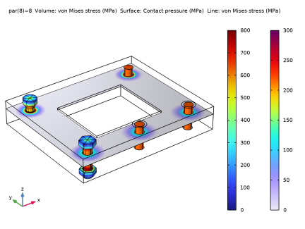
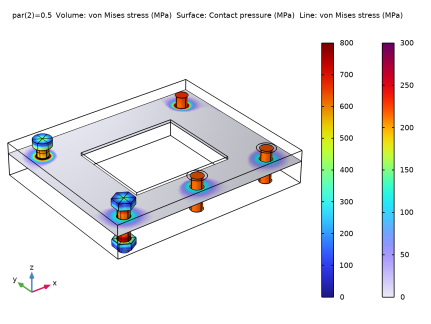
In the Settings window for 3D Plot Group, type Bolt Stress and Contact Pressure in the Label text field.
2
Volume 1
1
In the Model Builder window, expand the Bolt Stress and Contact Pressure node, then click Volume 1.
2
In the Settings window for Volume, locate the Expression section.
3
From the Unit list, choose MPa.
4
Click to expand the Range section. Select the Manual color range check box.
5
In the Maximum text field, type 800.
6
Locate the Coloring and Style section. Click  Change Color Table.
7
In the Color Table dialog box, select Rainbow>Rainbow in the tree.
8
Selection 1
1
Right-click Volume 1 and choose Selection.
2
3
In the Settings window for Selection, locate the Selection section.
4
From the Selection list, choose Bolts and Nuts.
Surface 1
1
In the Model Builder window, right-click Bolt Stress and Contact Pressure and choose Surface.
2
In the Settings window for Surface, click Replace Expression in the upper-right corner of the Expression section. From the menu, choose Component 1 (comp1)>Solid Mechanics>Contact>solid.Tn - Contact pressure - N/m².
3
Locate the Expression section. From the Unit list, choose MPa.
4
Locate the Coloring and Style section. Click  Change Color Table.
5
In the Color Table dialog box, select Rainbow>Prism in the tree.
6
7
In the Settings window for Surface, click to expand the Range section.
8
Select the Manual color range check box.
9
In the Maximum text field, type 300.
Deformation 1
1
Right-click Surface 1 and choose Deformation.
2
In the Settings window for Deformation, locate the Scale section.
3
Select the Scale factor check box.
Line 1
1
In the Model Builder window, expand the Results>Stress (beam) node.
2
Right-click Line 1 and choose Copy.
Line 1
1
In the Model Builder window, right-click Bolt Stress and Contact Pressure and choose Paste Line.
2
In the Settings window for Line, locate the Expression section.
3
From the Unit list, choose MPa.
4
Click to expand the Inherit Style section. From the Plot list, choose Volume 1.
5
Click the  Transparency button in the Graphics toolbar.
Study 1
In the Study toolbar, click  Compute.
Results
Bolt Stress and Contact Pressure
1
Click the  Show Grid button in the Graphics toolbar.
2
In the Bolt Stress and Contact Pressure toolbar, click  Plot.
Transverse Stress in the Bolt Planes
1
In the Home toolbar, click  Add Plot Group and choose 3D Plot Group.
2
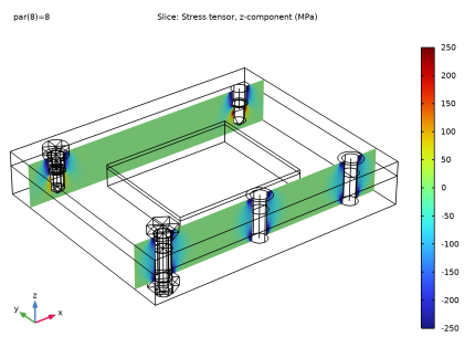
In the Settings window for 3D Plot Group, type Transverse Stress in the Bolt Planes in the Label text field.
Slice 1
1
Right-click Transverse Stress in the Bolt Planes and choose Slice.
2
In the Settings window for Slice, locate the Expression section.
3
In the Expression text field, type solid.sz.
4
From the Unit list, choose MPa.
5
Locate the Plane Data section. From the Plane list, choose ZX-planes.
6
From the Entry method list, choose Coordinates.
7
In the Y-coordinates text field, type 20 plateWidth-20.
8
Click to expand the Range section. Select the Manual color range check box.
9
In the Minimum text field, type -250.
10
In the Maximum text field, type 250.
Selection 1
1
Right-click Slice 1 and choose Selection.
2
3
In the Transverse Stress in the Bolt Planes toolbar, click  Plot.
Bolt Forces: Bolt Pretension 1 (Study 1) (solid)
1
In the Model Builder window, under Results click Bolt Forces: Bolt Pretension 1 (Study 1) (solid).
2
In the Bolt Forces: Bolt Pretension 1 (Study 1) (solid) toolbar, click  Evaluate.
Bolt Forces: Bolt Pretension 1 (Study 1) (beam)
1
In the Model Builder window, click Bolt Forces: Bolt Pretension 1 (Study 1) (beam).
2
In the Bolt Forces: Bolt Pretension 1 (Study 1) (beam) toolbar, click  Evaluate.
Solid Mechanics (solid)
Add the service load, a pressure inside the cavity.
In the Model Builder window, under Component 1 (comp1) click Solid Mechanics (solid).
Boundary Load 1
1
In the Physics toolbar, click  Boundaries and choose Boundary Load.
2
In the Settings window for Boundary Load, locate the Force section.
3
From the Load type list, choose Pressure.
4
In the p text field, type 4[MPa]*par.
5
Study 1
In case you need to recompute the pretensioning step, the pressure load should not be active there.
Step 1: Bolt Pretension
1
In the Model Builder window, under Study 1 click Step 1: Bolt Pretension.
2
In the Settings window for Bolt Pretension, locate the Physics and Variables Selection section.
3
Select the Modify model configuration for study step check box.
4
In the tree, select Component 1 (comp1)>Solid Mechanics (solid), Controls spatial frame>Boundary Load 1.
5
Root
Add a new study for the service load.
Add Study
1
In the Home toolbar, click  Add Study to open the Add Study window.
2
Go to the Add Study window.
3
Find the Studies subsection. In the Select Study tree, select General Studies>Stationary.
4
Study 2
Step 1: Stationary
1
In the Home toolbar, click  Add Study to close the Add Study window.
Study the effect of 20%, 50%, and 100% of the service load.
2
In the Model Builder window, under Study 2 click Step 1: Stationary.
3
In the Settings window for Stationary, click to expand the Study Extensions section.
4
Select the Auxiliary sweep check box.
5
6
Pick up the prestress solution from the previous study.
7
Click to expand the Values of Dependent Variables section. Find the Initial values of variables solved for subsection. From the Settings list, choose User controlled.
8
From the Method list, choose Solution.
9
From the Study list, choose Study 1, Bolt Pretension.
10
Find the Values of variables not solved for subsection. From the Settings list, choose User controlled.
11
From the Method list, choose Solution.
12
From the Study list, choose Study 1, Bolt Pretension.
Solution 2 (sol2)
1
In the Study toolbar, click  Show Default Solver.
2
In the Model Builder window, expand the Solution 2 (sol2) node.
3
In the Model Builder window, expand the Study 2>Solver Configurations>Solution 2 (sol2)>Dependent Variables 1 node, then click Rotation field (material and geometry frames) (comp1.beam.thLin).
4
In the Settings window for Field, locate the Scaling section.
5
From the Method list, choose Manual.
6
In the Scale text field, type 0.01.
7
In the Model Builder window, under Study 2>Solver Configurations>Solution 2 (sol2)>Dependent Variables 1 click Displacement field (material and geometry frames) (comp1.beam.uLin).
8
In the Settings window for Field, locate the Scaling section.
9
From the Method list, choose Manual.
10
In the Scale text field, type 0.001.
11
In the Model Builder window, expand the Study 2>Solver Configurations>Solution 2 (sol2)>Stationary Solver 1 node, then click Advanced.
12
In the Settings window for Advanced, locate the Assembly Settings section.
13
Clear the Reuse sparsity pattern check box.
14
In the Study toolbar, click  Compute.
Results
Bolt Stress and Contact Pressure, Service Load
1
In the Model Builder window, right-click Bolt Stress and Contact Pressure and choose Duplicate.
2
In the Settings window for 3D Plot Group, type Bolt Stress and Contact Pressure, Service Load in the Label text field.
Examine the results for different load levels.
3
Click to expand the Data section. From the Dataset list, choose Study 2/Solution 2 (sol2).
4
From the Parameter value (par) list, choose 0.2.
5
In the Bolt Stress and Contact Pressure, Service Load toolbar, click  Plot.
6
From the Parameter value (par) list, choose 0.5.
7
In the Bolt Stress and Contact Pressure, Service Load toolbar, click  Plot.
8
From the Parameter value (par) list, choose 1.
9
In the Bolt Stress and Contact Pressure, Service Load toolbar, click  Plot.
Evaluate the bolt forces.
Bolt Forces: Bolt Pretension 1 (Study 2) (solid)
1
In the Model Builder window, click Bolt Forces: Bolt Pretension 1 (Study 2) (solid).
2
In the Bolt Forces: Bolt Pretension 1 (Study 2) (solid) toolbar, click  Evaluate.
Bolt Forces: Bolt Pretension 1 (Study 2) (beam)
1
In the Model Builder window, click Bolt Forces: Bolt Pretension 1 (Study 2) (beam).
2
In the Bolt Forces: Bolt Pretension 1 (Study 2) (beam) toolbar, click  Evaluate.
Tightening Torque
Evaluate the required tightening torque for full prestress.
1
In the Results toolbar, click  Evaluation Group.
2
In the Settings window for Evaluation Group, type Tightening Torque in the Label text field.
Global Evaluation 1
1
Right-click Tightening Torque and choose Global Evaluation.
2
In the Settings window for Global Evaluation, click Replace Expression in the upper-right corner of the Expressions section. From the menu, choose Component 1 (comp1)>Solid Mechanics>Bolts>Bolt_1>solid.pblt1.sblt1.M_pre - Tightening torque - N·m.
Tightening Torque
1
In the Model Builder window, click Tightening Torque.
2
In the Settings window for Evaluation Group, locate the Data section.
3
From the Parameter selection (par) list, choose First.
4
In the Tightening Torque toolbar, click  Evaluate.