You are viewing the documentation for an older COMSOL version. The latest version is available here.
PDF

Axisymmetric Twist and Bending
Introduction
When using a 2D axisymmetric Solid Mechanics interface, the primary dependent variables are, by default, the displacements in the radial and axial directions, u and w. It is, however, possible to also include the displacement component in the circumferential direction, v, which opens up the possibility to model both twisting and bending deformations. The extension of a 2D model to solve for a true 3D displacement field is sometimes referred to as a 2.5D formulation.
The primary objective of this model is to show how to model twist and bending in 2D axisymmetry. A hollow axisymmetric shaft is subjected to different load cases, and the stress concentration factors are derived for each case. The analyses are performed both in 2D axisymmetry and 3D to demonstrate their equivalence. However, if the geometry allows it, modeling in 2D axisymmetry is generally preferable being computationally significantly cheaper as well as more convenient to set up.
Figure 1: Shaft geometry and relevant geometric properties.
Model Definition
The geometry of the hollow shaft is shown in Figure 1. The transition between the thicker and thinner sections is slightly smoothened by a fillet. The shaft is made of steel (see Table 1) and behaves linear elastically.
The wider end is fixed, while a load is applied at the narrow end. Three different load cases are examined:
1
2
3
In the transition region between the small and large shaft diameters, local stress concentrations are expected due to the disturbance in the stress field. For the three load cases, stress concentration factors are evaluated numerically in this model. In general, the geometrical stress concentration factor is defined as the ratio between the actual maximum stress, σmax, and the nominal stress, σnom, in the region where the stress field is disturbed:
Here, the nominal stress, σnom, is the stress computed from elementary theories. The stress concentration factors are defined as follows for the three load cases:
Axial extension: where
  Torsion: where
Bending: where
Here, Fz, Mt, and Mb are the applied force in the z direction, the torsional moment, and the bending moment, respectively. Furthermore, A, J, and I are the cross-section area, the torsional constant, and the area moment of inertia for the thinner section of the hollow shaft.
In order to solve for torsion and bending in 2D axisymmetry, the standard formulation has to be augmented by including the displacement in the circumferential direction, v, as a new dependent variable. By default, this circumferential displacement is assumed to be zero, and the extended 2D axisymmetric formulation must be turned on explicitly in COMSOL Multiphysics. Adding a new dependent variable increases the size of the system matrices slightly.
In addition to adding the displacement field component in the φ direction, the displacement gradient, u, is augmented to include the spatial variation of the circumferential displacement. The displacement gradient is a fundamental quantity used to define important variables such as strains and subsequently stresses. There can be alternative formulations of the displacement gradient depending on the chosen study type. In general, the gradient of the displacement field in a cylindrical coordinate system is defined as
Assuming that the displacement is constant in the circumferential direction, the derivatives with respect to φ become zero, and u simplifies to
This formulation, which allows a constant displacement around the circumference, is available for all study types.
For frequency-domain and eigenfrequency studies, the displacement field is allowed to have a periodic variation in the φ direction. This approach is sometimes referred to as a circumferential mode extension. The following complex-valued ansatz for the displacement field is assumed:
Here, m is the mode number. This ansatz allows periodic displacements in the circumferential direction, and it has two noteworthy special cases. The case of m = 0 corresponds to a constant circumferential displacement, and m = 1 allows a bending-type displacement. With the new ansatz, the displacement gradient becomes
This formulation is only available for frequency-domain and eigenfrequency studies, and it is only valid for small strains.
The assumed complex-valued displacement field has implications for how an excitation load should be applied when working with a cylindrical coordinate system since the force vector is to be entered according to the base vectors of the cylindrical system. In the corresponding 3D case, the bending load is applied as a total force acting in the positive X direction of the global Cartesian coordinate system. From a parallelogram of forces it can be shown that the force FX can be written in terms of force components expressed in the cylindrical system.
The force entered in the load feature acts directly on the displacement field, hence the force vector is implicitly multiplied by . Therefore, the load vector should be defined only as
which corresponds to a real-valued load FX acting in the X direction for m = 1.
Results and Discussion
The von Mises stress distribution is shown in Figure 2Figure 4 for the three load cases, that is, axial extension, torsion, and bending. The 2D axisymmetric solution closely matches the 3D solution for all cases.
To find the highest stress value in the region of interest, the stress intensification factors are evaluated using a maximum operator (see the evaluation group Stress Concentration Factors under the Results node of the Model Builder). Again, the computationally leaner 2D axisymmetric solution shows good agreement with the full 3D result. Axial extension produces the highest stress concentration factor, followed by bending and torsion.
Figure 2: von Mises stress for axial load as computed in 2D axisymmetry (left) and 3D.
Figure 3: von Mises stress for torsional load as computed in 2D axisymmetry (left) and 3D.
Figure 4: von Mises stress for bending load as computed in 2D axisymmetry (left) and 3D.
It is worth highlighting that the number of degrees of freedom (DOFs) is roughly 25 times higher for the 3D model, which directly affects assembly and solver time. When investigating stress concentrations, it is often of interest to examine effects of geometrical changes such as varying fillet or diameter sizes in between different shaft sections. Such geometrical investigations can easily be performed in COMSOL Multiphysics using parametric sweeps. The geometry needs to be rebuilt and remeshed, and the model needs to be re-solved. This can be done more efficiently with only a 2D geometry.
Notes About the COMSOL Implementation
The model is set up and solved for twice in order to show the equivalence between the 2D axisymmetric and full 3D formulations.
Bending deformations in 2D axisymmetry can only be computed in frequency-domain or in eigenfrequency studies. Therefore, a frequency-domain study is added with an excitation frequency of 0 Hz. This corresponds to a stationary analysis since the applied loads will have no time-harmonic part.
Note also that all three load cases could have been solved for with a single frequency-domain study. In this case, the azimuthal mode number would have had to be defined as
m = if(group.lg3, 1, 0)
Here, group.lg3 is the weight variable of load group 3 (bending). The variable is defined in the Study Extensions section when adding load cases. The above expression for m sets the azimuthal mode number to 0 for the first and second load cases (that is, axial extension and torsion) and to 1 for the third load case (that is, bending).
Application Library path: Structural_Mechanics_Module/Verification_Examples/axisymmetric_twist_and_bending
Modeling Instructions
From the File menu, choose New.
New
In the New window, click  Model Wizard.
Model Wizard
1
In the Model Wizard window, click  2D Axisymmetric.
2
In the Select Physics tree, select Structural Mechanics>Solid Mechanics (solid).
3
Click Add.
4
Click  Study.
5
In the Select Study tree, select General Studies>Stationary.
6
Global Definitions
Parameters 1
1
In the Model Builder window, under Global Definitions click Parameters 1.
2
In the Settings window for Parameters, locate the Parameters section.
3
Create a 2D shaft section as a global geometry part so that it can be referenced by the 2D axisymmetric and 3D components, respectively.
Shaft Section
1
In the Model Builder window, right-click Global Definitions and choose Geometry Parts>2D Part.
2
In the Settings window for Part, type Shaft Section in the Label text field.
3
Locate the Units section. From the Length unit list, choose mm.
Polygon 1 (pol1)
1
In the Geometry toolbar, click  Polygon.
2
In the Settings window for Polygon, locate the Coordinates section.
3
Fillet 1 (fil1)
1
In the Geometry toolbar, click  Fillet.
2
On the object pol1, select Point 3 only.
3
In the Settings window for Fillet, locate the Radius section.
4
In the Radius text field, type 1.
Fillet 2 (fil2)
1
In the Geometry toolbar, click  Fillet.
2
On the object fil1, select Point 3 only.
3
In the Settings window for Fillet, locate the Radius section.
4
In the Radius text field, type 2.
5
In the Geometry toolbar, click  Build All.
Add Material
1
In the Home toolbar, click  Add Material to open the Add Material window.
2
Go to the Add Material window.
3
In the tree, select Built-in>Structural steel.
4
Right-click and choose Add to Global Materials.
5
In the Home toolbar, click  Add Material to close the Add Material window.
Global Definitions
Axial Extension
1
Right-click Global Definitions and choose Load and Constraint Groups>Load Group.
2
In the Settings window for Load Group, type Axial Extension in the Label text field.
Torsion
1
In the Model Builder window, right-click Load and Constraint Groups and choose Load Group.
2
In the Settings window for Load Group, type Torsion in the Label text field.
Bending
1
Right-click Load and Constraint Groups and choose Load Group.
2
In the Settings window for Load Group, type Bending in the Label text field.
Geometry 1
1
In the Model Builder window, under Component 1 (comp1) click Geometry 1.
2
In the Settings window for Geometry, locate the Units section.
3
From the Length unit list, choose mm.
Shaft Section 1 (pi1)
In the Geometry toolbar, click  Parts and choose Shaft Section.
Materials
Material Link 1 (matlnk1)
In the Model Builder window, under Component 1 (comp1) right-click Materials and choose More Materials>Material Link.
Next, include the circumferential displacement as a new dependent variable to allow twisting deformations. In addition, enable the mode extension with mode number 1, which allows to compute bending deformations in frequency domain.
Solid Mechanics (solid)
1
In the Settings window for Solid Mechanics, locate the Axial Symmetry Approximation section.
2
Select the Include circumferential displacement check box.
3
Find the Time-harmonic subsection. Select the Circumferential mode extension check box.
4
In the m text field, type 1.
Fixed Constraint 1
1
Right-click Component 1 (comp1)>Solid Mechanics (solid) and choose Fixed Constraint.
2
Boundary Load: Axial Extension
1
In the Physics toolbar, click  Boundaries and choose Boundary Load.
2
In the Settings window for Boundary Load, type Boundary Load: Axial Extension in the Label text field.
3
4
Locate the Force section. From the Load type list, choose Total force.
5
Specify the Ftot vector as
6
In the Physics toolbar, click  Load Group and choose Axial Extension.
Boundary Load: Torsion
1
In the Physics toolbar, click  Boundaries and choose Boundary Load.
2
In the Settings window for Boundary Load, type Boundary Load: Torsion in the Label text field.
3
4
Locate the Force section. From the Load type list, choose Total force.
5
Specify the Ftot vector as
6
In the Physics toolbar, click  Load Group and choose Torsion.
Boundary Load: Bending
1
In the Physics toolbar, click  Boundaries and choose Boundary Load.
The bending force will be active only in frequency domain, where a complex-valued displacement field is assumed. The real part of the force should act only in x direction when interpreted in a Cartesian coordinate system. The coordinate transformation from the cylindrical to Cartesian system requires the force to be complex-valued.
2
In the Settings window for Boundary Load, type Boundary Load: Bending in the Label text field.
3
4
Locate the Force section. From the Load type list, choose Total force.
5
Specify the Ftot vector as
6
In the Physics toolbar, click  Load Group and choose Bending.
Mesh 1
Free Triangular 1
In the Mesh toolbar, click  Free Triangular.
Distribution 1
1
Right-click Free Triangular 1 and choose Distribution.
2
3
In the Settings window for Distribution, locate the Distribution section.
4
In the Number of elements text field, type 20.
Size
1
In the Model Builder window, under Component 1 (comp1)>Mesh 1 click Size.
2
In the Settings window for Size, locate the Element Size section.
3
From the Predefined list, choose Finer.
4
Click  Build All.
Definitions
Maximum 1 (maxop1)
1
In the Definitions toolbar, click  Nonlocal Couplings and choose Maximum.
2
In the Settings window for Maximum, type max2Daxi in the Operator name text field.
3
Locate the Source Selection section. From the Geometric entity level list, choose Boundary.
4
Add Component
In the Model Builder window, right-click the root node and choose Add Component>3D.
Geometry 2
1
In the Settings window for Geometry, locate the Units section.
2
From the Length unit list, choose mm.
Work Plane 1 (wp1)
1
In the Geometry toolbar, click  Work Plane.
2
In the Settings window for Work Plane, locate the Plane Definition section.
3
From the Plane list, choose xz-plane.
Work Plane 1 (wp1)>Plane Geometry
In the Model Builder window, click Plane Geometry.
Work Plane 1 (wp1)>Shaft Section 1 (pi1)
In the Work Plane toolbar, click  Parts and choose Shaft Section.
Revolve 1 (rev1)
1
In the Model Builder window, under Component 2 (comp2)>Geometry 2 right-click Work Plane 1 (wp1) and choose Revolve.
2
In the Settings window for Revolve, click  Build All Objects.
Definitions (comp2)
Cylindrical System (Material Frame)
1
In the Definitions toolbar, click  Coordinate Systems and choose Cylindrical System.
2
In the Settings window for Cylindrical System, type Cylindrical System (Material Frame) in the Label text field.
3
Locate the Coordinate Names section. From the Frame list, choose Material  (X, Y, Z).
Add Physics
1
In the Home toolbar, click  Add Physics to open the Add Physics window.
2
Go to the Add Physics window.
3
In the tree, select Structural Mechanics>Solid Mechanics (solid).
4
Click Add to Component 2 in the window toolbar.
5
In the Home toolbar, click  Add Physics to close the Add Physics window.
Materials
Material Link 2 (matlnk2)
In the Model Builder window, under Component 2 (comp2) right-click Materials and choose More Materials>Material Link.
Solid Mechanics 2 (solid2)
Linear Elastic Material 1
1
In the Settings window for Linear Elastic Material, locate the Coordinate System Selection section.
2
From the Coordinate system list, choose Cylindrical System (Material Frame) (sys3).
3
In the Model Builder window, click Solid Mechanics 2 (solid2).
Fixed Constraint 1
1
In the Physics toolbar, click  Boundaries and choose Fixed Constraint.
2
Boundary Load: Axial Extension
1
In the Physics toolbar, click  Boundaries and choose Boundary Load.
2
In the Settings window for Boundary Load, type Boundary Load: Axial Extension in the Label text field.
3
4
Locate the Force section. From the Load type list, choose Total force.
5
Specify the Ftot vector as
6
In the Physics toolbar, click  Load Group and choose Axial Extension.
Boundary Load: Torsion
1
In the Physics toolbar, click  Boundaries and choose Boundary Load.
2
In the Settings window for Boundary Load, type Boundary Load: Torsion in the Label text field.
3
4
Locate the Coordinate System Selection section. From the Coordinate system list, choose Cylindrical System (Material Frame) (sys3).
5
Locate the Force section. From the Load type list, choose Total force.
6
Specify the Ftot vector as
7
In the Physics toolbar, click  Load Group and choose Torsion.
Boundary Load: Bending
1
In the Physics toolbar, click  Boundaries and choose Boundary Load.
2
In the Settings window for Boundary Load, type Boundary Load: Bending in the Label text field.
3
4
Locate the Force section. From the Load type list, choose Total force.
5
Specify the Ftot vector as
6
In the Physics toolbar, click  Load Group and choose Bending.
Definitions (comp2)
Maximum 2 (maxop2)
1
In the Definitions toolbar, click  Nonlocal Couplings and choose Maximum.
2
In the Settings window for Maximum, locate the Source Selection section.
3
From the Geometric entity level list, choose Boundary.
4
In the Operator name text field, type max3D.
5
Mesh 2
Free Triangular 1
1
In the Mesh toolbar, click  Boundary and choose Free Triangular.
2
Distribution 1
1
Right-click Free Triangular 1 and choose Distribution.
2
3
In the Settings window for Distribution, locate the Distribution section.
4
In the Number of elements text field, type 20.
Swept 1
In the Mesh toolbar, click  Swept.
Size
1
In the Model Builder window, click Size.
2
In the Settings window for Size, locate the Element Size section.
3
From the Predefined list, choose Extra fine.
4
Click  Build All.
Study 1: Axial Extension & Torsion
1
In the Model Builder window, click Study 1.
2
In the Settings window for Study, type Study 1: Axial Extension & Torsion in the Label text field.
Step 1: Stationary
1
In the Model Builder window, under Study 1: Axial Extension & Torsion click Step 1: Stationary.
2
In the Settings window for Stationary, click to expand the Study Extensions section.
3
Select the Define load cases check box.
4
5
6
7
8
In the Home toolbar, click  Compute.
Add Study
1
In the Home toolbar, click  Add Study to open the Add Study window.
2
Go to the Add Study window.
3
Find the Studies subsection. In the Select Study tree, select General Studies>Frequency Domain.
4
Click Add Study in the window toolbar.
5
In the Home toolbar, click  Add Study to close the Add Study window.
Bending in 2D axisymmetry requires a special ansatz for the displacement field which is only available for frequency-domain (and eigenfrequency) studies. In order to solve for a stationary response using a frequency-domain study, set the target frequency to 0.
Study 2: Bending
1
In the Model Builder window, click Study 2.
2
In the Settings window for Study, type Study 2: Bending in the Label text field.
Step 1: Frequency Domain
1
In the Model Builder window, under Study 2: Bending click Step 1: Frequency Domain.
2
In the Settings window for Frequency Domain, locate the Study Settings section.
3
In the Frequencies text field, type 0.
4
Click to expand the Study Extensions section. Select the Define load cases check box.
5
6
7
In the Home toolbar, click  Compute.
Results
Stress: Axial Extension & Torsion (2D axi & 3D)
1
In the Model Builder window, under Results click Stress, 3D (solid).
2
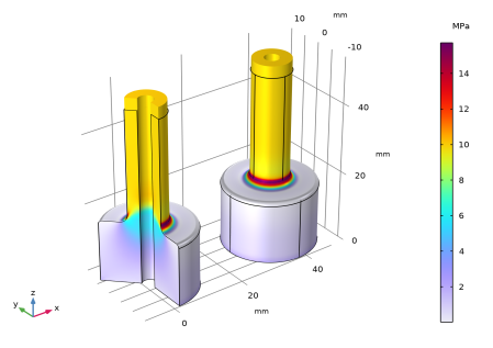
In the Settings window for 3D Plot Group, type Stress: Axial Extension & Torsion (2D axi & 3D) in the Label text field.
3
Click to expand the Title section. From the Title type list, choose None.
4
Locate the Color Legend section. Select the Show units check box.
Surface 1
1
In the Model Builder window, expand the Stress: Axial Extension & Torsion (2D axi & 3D) node, then click Surface 1.
2
In the Settings window for Surface, locate the Expression section.
3
From the Unit list, choose MPa.
Surface 2
1
In the Model Builder window, right-click Stress: Axial Extension & Torsion (2D axi & 3D) and choose Surface.
2
In the Settings window for Surface, locate the Data section.
3
From the Dataset list, choose Study 1: Axial Extension & Torsion/Solution 1 (2) (sol1).
4
From the Solution parameters list, choose From parent.
5
Locate the Expression section. In the Expression text field, type solid2.mises.
6
From the Unit list, choose MPa.
7
Click to expand the Inherit Style section. From the Plot list, choose Surface 1.
Deformation 1
Right-click Surface 2 and choose Deformation.
Translation 1
1
In the Model Builder window, right-click Surface 2 and choose Translation.
2
In the Settings window for Translation, locate the Translation section.
3
In the x text field, type 3*R1.
4
Clear the Apply to dataset edges check box.
Stress: Axial Extension & Torsion (2D axi & 3D)
1
In the Model Builder window, under Results click Stress: Axial Extension & Torsion (2D axi & 3D).
2
In the Settings window for 3D Plot Group, click  Plot First.
3
Click  Plot Next.
Stress: Bending (2D axi & 3D)
1
In the Model Builder window, expand the Results>Stress, 3D (solid) 1 node, then click Stress, 3D (solid) 1.
2
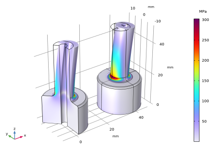
In the Settings window for 3D Plot Group, type Stress: Bending (2D axi & 3D) in the Label text field.
3
Locate the Title section. From the Title type list, choose None.
4
Locate the Color Legend section. Select the Show units check box.
Surface 1
1
In the Model Builder window, click Surface 1.
2
In the Settings window for Surface, locate the Expression section.
3
In the Expression text field, type solid.mises.
4
From the Unit list, choose MPa.
Surface 2
1
In the Model Builder window, right-click Stress: Bending (2D axi & 3D) and choose Surface.
2
In the Settings window for Surface, locate the Data section.
3
From the Dataset list, choose Study 2: Bending/Solution 2 (4) (sol2).
4
Locate the Expression section. In the Expression text field, type solid2.mises.
5
From the Unit list, choose MPa.
6
Locate the Inherit Style section. From the Plot list, choose Surface 1.
Deformation 1
Right-click Surface 2 and choose Deformation.
Translation 1
1
In the Model Builder window, right-click Surface 2 and choose Translation.
2
In the Settings window for Translation, locate the Translation section.
3
In the x text field, type 3*R1.
4
Clear the Apply to dataset edges check box.
Stress Concentration Factors
1
In the Results toolbar, click  Evaluation Group.
2
In the Settings window for Evaluation Group, type Stress Concentration Factors in the Label text field.
3
Locate the Data section. From the Dataset list, choose None.
4
Locate the Transformation section. Select the Transpose check box.
5
Click to expand the Format section. From the Include parameters list, choose Off.
Global Evaluation 1
1
Right-click Stress Concentration Factors and choose Global Evaluation.
2
In the Settings window for Global Evaluation, locate the Data section.
3
From the Dataset list, choose Study 1: Axial Extension & Torsion/Solution 1 (1) (sol1).
4
From the Parameter selection (Load case) list, choose First.
5
Locate the Expressions section. In the table, enter the following settings:
Global Evaluation 2
1
In the Model Builder window, right-click Stress Concentration Factors and choose Global Evaluation.
2
In the Settings window for Global Evaluation, locate the Data section.
3
From the Dataset list, choose Study 1: Axial Extension & Torsion/Solution 1 (1) (sol1).
4
From the Parameter selection (Load case) list, choose Last.
5
Locate the Expressions section. In the table, enter the following settings:
The local stress Sl23 in 3D represents the shear stress Sϕz, as a cylindrical system was selected in the Coordinate System Selection in the Linear Elastic Material node.
Global Evaluation 3
1
Right-click Stress Concentration Factors and choose Global Evaluation.
2
In the Settings window for Global Evaluation, locate the Data section.
3
From the Dataset list, choose Study 2: Bending/Solution 2 (3) (sol2).
4
From the Parameter selection (freq) list, choose Last.
5
From the Parameter selection (Load case) list, choose Last.
6
Locate the Expressions section. In the table, enter the following settings:
7
In the Stress Concentration Factors toolbar, click  Evaluate.