|
|
|
|
1
|
|
2
|
|
3
|
Click Add.
|
|
4
|
Click
|
|
5
|
|
6
|
Click
|
|
1
|
|
2
|
|
3
|
|
1
|
|
2
|
|
3
|
|
4
|
Browse to the model’s Application Libraries folder and double-click the file schrodinger_poisson_nanowire_param.txt.
|
|
1
|
In the Model Builder window, under Component 1 (comp1) right-click Definitions and choose Variables.
|
|
2
|
|
3
|
|
4
|
Browse to the model’s Application Libraries folder and double-click the file schrodinger_poisson_nanowire_var.txt.
|
|
1
|
|
2
|
|
1
|
In the Model Builder window, under Component 1 (comp1) right-click Materials and choose Blank Material.
|
|
2
|
|
1
|
|
2
|
|
3
|
|
1
|
In the Model Builder window, under Component 1 (comp1)>Schrödinger Equation (schr) click Effective Mass 1.
|
|
2
|
|
3
|
|
1
|
|
2
|
|
3
|
|
1
|
|
3
|
|
4
|
|
5
|
|
6
|
In the Show More Options dialog box, in the tree, select the check box for the node Physics>Advanced Physics Options.
|
|
7
|
Click OK.
|
|
8
|
|
9
|
|
1
|
|
2
|
In the Settings window for Space Charge Density, type Space Charge Density 1: Ionized dopants in the Label text field.
|
|
3
|
|
4
|
|
1
|
|
2
|
In the Settings window for Space Charge Density, type Space Charge Density 2: Thomas Fermi in the Label text field.
|
|
3
|
|
4
|
|
1
|
In the Model Builder window, under Component 1 (comp1)>Multiphysics click Schrödinger-Poisson Coupling 1 (schrp1).
|
|
2
|
|
3
|
|
4
|
|
5
|
|
6
|
|
7
|
|
1
|
|
2
|
|
3
|
|
1
|
|
2
|
|
1
|
|
2
|
|
3
|
|
4
|
|
5
|
|
1
|
|
2
|
|
3
|
Find the Studies subsection. In the Select Study tree, select Preset Studies for Selected Multiphysics>Schrödinger-Poisson.
|
|
4
|
|
5
|
|
1
|
|
2
|
|
3
|
|
4
|
|
5
|
Locate the Physics and Variables Selection section. Select the Modify model configuration for study step check box.
|
|
6
|
|
7
|
Click
|
|
8
|
Click to expand the Values of Dependent Variables section. Find the Initial values of variables solved for subsection. From the Settings list, choose User controlled.
|
|
9
|
|
10
|
|
11
|
|
12
|
Click
|
|
14
|
|
15
|
|
16
|
|
1
|
|
2
|
From the Dataset list, choose Study 2: Schrödinger-Poisson/Solution Store: Store Wave Function (sol4).
|
|
3
|
|
1
|
In the Model Builder window, right-click Compare n and V with Previous Iteration (schrp1) and choose Move Up four times.
|
|
2
|
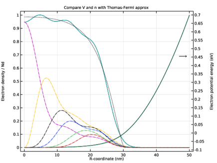
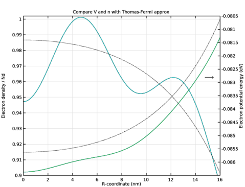
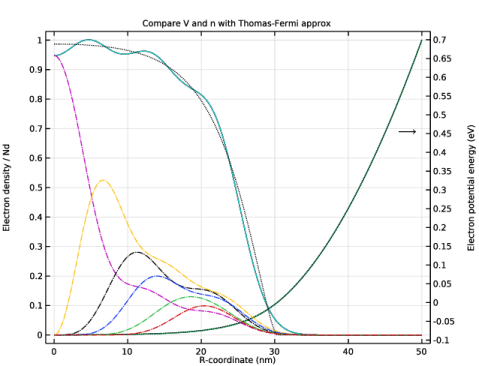
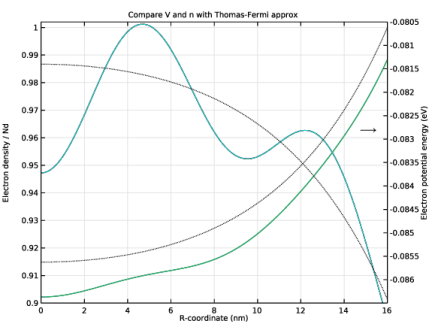
In the Settings window for 1D Plot Group, type Compare V and n with Thomas-Fermi approx in the Label text field.
|
|
3
|
Click to expand the Title section. In the Title text area, type Compare V and n with Thomas-Fermi approx.
|
|
4
|
|
5
|
|
1
|
In the Model Builder window, expand the Compare V and n with Thomas-Fermi approx node, then click Potential Energy.
|
|
2
|
|
3
|
|
4
|
|
1
|
In the Model Builder window, under Results>Compare V and n with Thomas-Fermi approx click Potential Energy from Previous Iteration.
|
|
2
|
In the Settings window for Line Graph, type Electron Potential Energy from Previous Iteration in the Label text field.
|
|
3
|
|
4
|
Select the Description check box. In the associated text field, type Electron Potential Energy, Previous Iteration.
|
|
1
|
In the Model Builder window, under Results>Compare V and n with Thomas-Fermi approx click Particle Density from Weighted Sum.
|
|
2
|
In the Settings window for Line Graph, type Electron Density from Weighted Sum in the Label text field.
|
|
3
|
|
4
|
Select the Description check box. In the associated text field, type Electron Density, Weighted Sum.
|
|
1
|
In the Model Builder window, under Results>Compare V and n with Thomas-Fermi approx click Particle Density.
|
|
2
|
|
3
|
|
4
|
|
1
|
In the Model Builder window, under Results>Compare V and n with Thomas-Fermi approx click Particle Density from Previous Iteration.
|
|
2
|
In the Settings window for Line Graph, type Electron Density from Previous Iteration in the Label text field.
|
|
3
|
|
4
|
Select the Description check box. In the associated text field, type Electron Density, Previous Iteration.
|
|
1
|
|
2
|
In the Settings window for Line Graph, type Electron Density from Thomas-Fermi Approx in the Label text field.
|
|
3
|
|
4
|
|
5
|
|
6
|
Click to expand the Coloring and Style section. Find the Line style subsection. From the Line list, choose Dotted.
|
|
7
|
|
1
|
|
2
|
In the Settings window for Line Graph, type Electron Potential Energy from Thomas-Fermi Approx in the Label text field.
|
|
3
|
|
4
|
|
5
|
|
1
|
In the Model Builder window, right-click Compare V and n with Thomas-Fermi approx and choose Annotation.
|
|
2
|
|
3
|
|
4
|
|
5
|
|
6
|
|
7
|
|
8
|
|
1
|
In the Model Builder window, expand the Study 2: Schrödinger-Poisson>Solver Configurations>Solution 2 (sol2)>Stationary Solver 2: Solve for Electric Potential node, then click Fully Coupled 1.
|
|
2
|
|
3
|
Select the Plot check box.
|
|
4
|
|
5
|
|
1
|
|
2
|
|
3
|
|
4
|
|
5
|
|
6
|
|
7
|
|
8
|
|
9
|
|
10
|
|
1
|
In the Model Builder window, expand the Compare V and n with Thomas-Fermi approx 1 node, then click Annotation 1.
|
|
2
|
|
3
|
|
4
|
|
5
|
|
1
|
In the Model Builder window, right-click Electron Density from Thomas-Fermi Approx and choose Duplicate.
|
|
2
|
|
3
|
Locate the y-Axis Data section. In the Expression text field, type sum(withsol('sol4',schrp1.ni,setval(m,0),setind(lambda,jj)),jj,1,4)/Nd.
|
|
4
|
|
5
|
Locate the Coloring and Style section. Find the Line style subsection. From the Line list, choose Dash-dot.
|
|
6
|
|
1
|
|
2
|
|
3
|
Locate the y-Axis Data section. In the Expression text field, type sum(withsol('sol4',schrp1.ni,setval(m,1),setind(lambda,jj)),jj,1,4)/Nd.
|
|
4
|
|
1
|
|
2
|
|
3
|
Locate the y-Axis Data section. In the Expression text field, type sum(withsol('sol4',schrp1.ni,setval(m,2),setind(lambda,jj)),jj,1,4)/Nd.
|
|
4
|
|
1
|
|
2
|
|
3
|
Locate the y-Axis Data section. In the Expression text field, type sum(withsol('sol4',schrp1.ni,setval(m,3),setind(lambda,jj)),jj,1,3)/Nd.
|
|
4
|
|
1
|
|
2
|
|
3
|
Locate the y-Axis Data section. In the Expression text field, type sum(withsol('sol4',schrp1.ni,setval(m,4),setind(lambda,jj)),jj,1,3)/Nd.
|
|
4
|
|
1
|
|
2
|
|
3
|
Locate the y-Axis Data section. In the Expression text field, type sum(withsol('sol4',schrp1.ni,setval(m,5),setind(lambda,jj)),jj,1,2)/Nd.
|
|
4
|
|
5
|
|
1
|
|
2
|
In the Settings window for Point Evaluation, type Point Evaluation 1: check charge neutrality in the Label text field.
|
|
3
|
Locate the Data section. From the Dataset list, choose Study 2: Schrödinger-Poisson/Solution 2 (sol2).
|
|
5
|
Locate the Expressions section. In the table, enter the following settings:
|
|
6
|
Click
|