|
|
|
|
1
|
|
2
|
|
3
|
Click Add.
|
|
4
|
|
5
|
Click Add.
|
|
6
|
Click
|
|
7
|
In the Select Study tree, select Preset Studies for Some Physics Interfaces>Semiconductor Equilibrium.
|
|
8
|
Click
|
|
1
|
|
2
|
|
3
|
|
1
|
|
2
|
|
1
|
|
2
|
|
3
|
Find the Intervals subsection. In the table, enter the following settings:
|
|
4
|
|
5
|
|
1
|
|
2
|
|
1
|
In the Model Builder window, under Component 1 (comp1) right-click Definitions and choose Variables.
|
|
2
|
|
1
|
|
2
|
|
3
|
|
4
|
|
5
|
|
1
|
|
2
|
|
3
|
|
1
|
In the Model Builder window, under Component 1 (comp1)>Semiconductor (semi) click Semiconductor Material Model 1.
|
|
2
|
|
3
|
|
4
|
|
1
|
|
2
|
In the Settings window for Analytic Doping Model, type Analytic Doping Model 1: Intrinsic in the Label text field.
|
|
3
|
|
4
|
|
1
|
|
2
|
In the Settings window for Geometric Doping Model, type Geometric Doping Model 1: P-plus in the Label text field.
|
|
3
|
|
4
|
Locate the Distribution section. From the Profile away from the boundary list, choose Error function (erf).
|
|
5
|
|
6
|
|
7
|
|
1
|
|
2
|
In the Settings window for Geometric Doping Model, type Geometric Doping Model 2: N-plus in the Label text field.
|
|
3
|
|
4
|
|
1
|
In the Model Builder window, expand the Component 1 (comp1)>Semiconductor (semi)>Geometric Doping Model 1: P-plus node, then click Boundary Selection for Doping Profile 1.
|
|
1
|
In the Model Builder window, expand the Component 1 (comp1)>Semiconductor (semi)>Geometric Doping Model 2: N-plus node, then click Boundary Selection for Doping Profile 1.
|
|
1
|
|
2
|
In the Settings window for Trap-Assisted Recombination, type Trap-Assisted Recombination 1: SRH in the Label text field.
|
|
3
|
|
4
|
Locate the Shockley-Read-Hall Recombination section. From the τn list, choose User defined. In the associated text field, type tau.
|
|
5
|
|
1
|
|
2
|
|
3
|
|
4
|
Locate the Impact Ionization Generation section. From the Impact ionization model list, choose User-defined.
|
|
5
|
|
6
|
|
1
|
|
2
|
In the Settings window for User-Defined Generation, type User-Defined Generation 1: Radiation effect in the Label text field.
|
|
3
|
|
4
|
|
5
|
|
1
|
|
2
|
|
1
|
|
2
|
|
4
|
|
1
|
|
2
|
|
3
|
|
1
|
|
2
|
|
3
|
|
1
|
|
2
|
In the Settings window for Study, type Study 1a: Ramp V0 with field-independent mobility in the Label text field.
|
|
1
|
In the Model Builder window, under Study 1a: Ramp V0 with field-independent mobility click Step 1: Semiconductor Equilibrium.
|
|
2
|
In the Settings window for Semiconductor Equilibrium, locate the Physics and Variables Selection section.
|
|
3
|
|
1
|
|
2
|
|
3
|
|
4
|
|
5
|
|
6
|
Click
|
|
8
|
Click
|
|
10
|
|
11
|
|
12
|
|
1
|
|
2
|
|
3
|
In the Model Builder window, expand the Study 1a: Ramp V0 with field-independent mobility>Solver Configurations>Solution 1 (sol1)>Stationary Solver 2 node, then click Parametric 1.
|
|
4
|
|
5
|
|
6
|
|
1
|
|
2
|
|
3
|
Find the Physics interfaces in study subsection. In the table, clear the Solve check box for Events (ev).
|
|
4
|
|
5
|
|
6
|
|
1
|
|
2
|
Find the Initial values of variables solved for subsection. From the Settings list, choose User controlled.
|
|
3
|
|
4
|
|
5
|
|
6
|
|
1
|
|
2
|
|
3
|
Click
|
|
5
|
Click
|
|
7
|
|
8
|
In the Settings window for Study, type Study 1b: Ramp V0 with full mobility model in the Label text field.
|
|
9
|
|
1
|
|
2
|
|
3
|
|
1
|
|
2
|
|
3
|
|
4
|
|
5
|
|
6
|
|
7
|
|
1
|
|
2
|
|
3
|
|
4
|
|
5
|
|
6
|
|
7
|
|
8
|
|
9
|
|
10
|
|
1
|
|
2
|
|
3
|
|
4
|
|
5
|
|
6
|
|
1
|
|
2
|
|
3
|
|
4
|
Clear the Description check box.
|
|
5
|
|
6
|
|
7
|
|
8
|
|
1
|
|
2
|
In the Settings window for 1D Plot Group, type Fig. 4B Electric Field Distribution in the Label text field.
|
|
3
|
|
4
|
|
5
|
|
1
|
In the Model Builder window, expand the Fig. 4B Electric Field Distribution node, then click Line Graph 1.
|
|
2
|
|
3
|
|
4
|
|
5
|
|
1
|
|
2
|
|
3
|
Find the Physics interfaces in study subsection. In the table, clear the Solve check box for Events (ev).
|
|
4
|
|
5
|
|
6
|
|
1
|
|
2
|
In the Settings window for Study, type Study 2: Steady-state radiation effect in the Label text field.
|
|
3
|
|
1
|
|
2
|
|
3
|
Find the Initial values of variables solved for subsection. From the Settings list, choose User controlled.
|
|
4
|
|
5
|
|
6
|
|
7
|
|
8
|
Click
|
|
10
|
Click
|
|
1
|
|
2
|
|
3
|
In the Model Builder window, expand the Study 2: Steady-state radiation effect>Solver Configurations>Solution 12 (sol12)>Stationary Solver 1 node, then click Fully Coupled 1.
|
|
4
|
|
5
|
|
6
|
|
7
|
In the Model Builder window, under Study 2: Steady-state radiation effect>Solver Configurations>Solution 12 (sol12)>Stationary Solver 1 click Parametric 1.
|
|
8
|
|
9
|
|
10
|
|
11
|
|
12
|
|
13
|
In the Model Builder window, under Study 2: Steady-state radiation effect>Solver Configurations>Solution 12 (sol12)>Stationary Solver 1 click Fully Coupled 1.
|
|
14
|
|
15
|
|
16
|
|
17
|
|
18
|
|
1
|
|
2
|
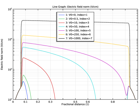
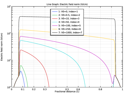
In the Settings window for 1D Plot Group, type Fig. 5A Steady-State Electric Field Distribution vs. Dose Rate in the Label text field.
|
|
3
|
Locate the Data section. From the Dataset list, choose Study 2: Steady-state radiation effect/Solution 12 (sol12).
|
|
4
|
|
5
|
|
6
|
|
1
|
|
2
|
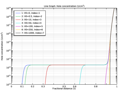
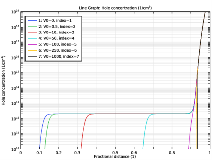
In the Settings window for 1D Plot Group, type Fig. 5B Steady-State Hole Distribution vs. Dose Rate in the Label text field.
|
|
3
|
Locate the Data section. From the Dataset list, choose Study 2: Steady-state radiation effect/Solution 12 (sol12).
|
|
4
|
|
5
|
|
6
|
|
7
|
|
1
|
|
2
|
|
3
|
Locate the Data section. From the Dataset list, choose Study 1b: Ramp V0 with full mobility model/Parametric Solutions 1 (sol4).
|
|
4
|
|
5
|
|
6
|
|
7
|
Select the y-axis label check box. In the associated text field, type Mobility (cm<sup>2</sup>/V-s).
|
|
8
|
|
9
|
|
10
|
|
11
|
|
12
|
|
13
|
|
14
|
|
1
|
|
2
|
|
3
|
|
4
|
|
5
|
|
6
|
|
7
|
Click to expand the Coloring and Style section. Find the Line style subsection. From the Line list, choose None.
|
|
8
|
|
9
|
|
10
|
|
1
|
|
2
|
|
3
|
|
4
|
Locate the Coloring and Style section. Find the Line markers subsection. From the Marker list, choose Cycle (reset).
|
|
1
|
|
2
|
|
3
|
|
4
|
|
5
|
|
6
|
|
7
|
|
1
|
|
2
|
|
3
|
|
4
|
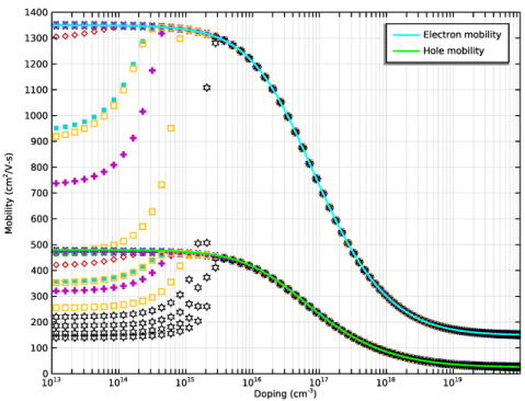
Locate the y-Axis Data section. In the Expression text field, type mun0[V*s/cm^2]/(1+81*10^logNDt/(10^logNDt+3.24e18))^0.5.
|
|
5
|
|
6
|
|
7
|
|
8
|
|
9
|
|
10
|
|
11
|
|
12
|
Select the Description check box.
|
|
1
|
|
2
|
|
3
|
|
4
|
|
5
|
|
6
|
|
1
|
|
2
|
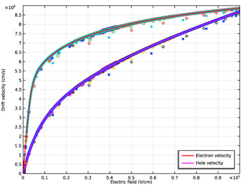
In the Settings window for 1D Plot Group, type Fig. 2B Velocity vs. Electric Field in the Label text field.
|
|
3
|
Locate the Data section. From the Dataset list, choose Study 2: Steady-state radiation effect/Solution 12 (sol12).
|
|
4
|
|
5
|
|
6
|
|
7
|
|
8
|
|
9
|
|
10
|
|
1
|
In the Model Builder window, expand the Fig. 2B Velocity vs. Electric Field node, then click Line Graph 1.
|
|
2
|
|
3
|
|
4
|
|
5
|
|
6
|
Clear the Description check box.
|
|
1
|
|
2
|
|
3
|
|
4
|
|
5
|
|
6
|
Clear the Description check box.
|
|
1
|
|
2
|
|
3
|
|
4
|
|
5
|
|
1
|
|
2
|
|
3
|
|
4
|
Locate the y-Axis Data section. In the Expression text field, type E1*mun0[V*s/cm^2]/(1+(E1/8e3)^4.9*(E1+1.64e5)/(E1+1))^(1/4.9).
|
|
5
|
|
6
|
|
7
|
|
8
|
|
1
|
|
2
|
|
3
|
|
4
|
Locate the y-Axis Data section. In the Expression text field, type E1*mup0[V*s/cm^2]/(1+(E1/8.72e4)^1.15*(E1+8.51e5)/(E1+8.12e4))^(1/1.15).
|
|
5
|
|
6
|
|
7
|
|
8
|
|
9
|
|
1
|
|
2
|
|
3
|
|
4
|
|
5
|
|
1
|
|
2
|
|
3
|
In the Output times text field, type 0 0.1 0.2 0.3 0.5 0.6 0.8 1 1.3 1.7 2 2.4 3 3.5 4 4.3 4.7 5 6 7 8 10.
|
|
4
|
|
5
|
|
6
|
Click to expand the Values of Dependent Variables section. Find the Initial values of variables solved for subsection. From the Settings list, choose User controlled.
|
|
7
|
|
8
|
|
9
|
|
10
|
Click
|
|
12
|
|
13
|
|
14
|
|
1
|
|
2
|
|
3
|
|
4
|
|
5
|
|
1
|
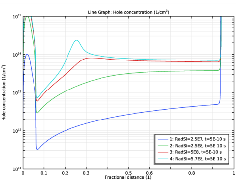
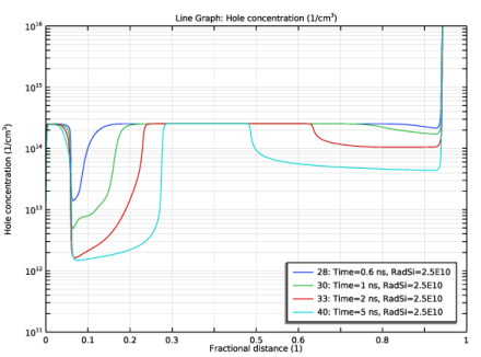
In the Model Builder window, right-click Fig. 5B Steady-State Hole Distribution vs. Dose Rate and choose Duplicate.
|
|
2
|
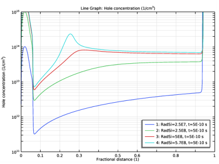
In the Settings window for 1D Plot Group, type Fig. 7A Hole Distribution at Several Times in the Label text field.
|
|
3
|
Locate the Data section. From the Dataset list, choose Study 3: Pulsed radiation effect/Solution 13 (sol13).
|
|
4
|
|
5
|
|
6
|
|
7
|
|
8
|
|
1
|
|
2
|
|
3
|
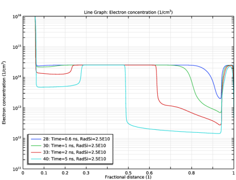
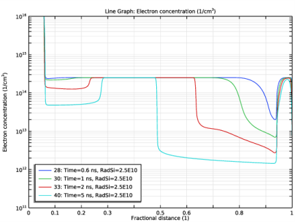
In the Settings window for 1D Plot Group, type Fig. 7B Electron Distribution at Several Times in the Label text field.
|
|
4
|
|
1
|
|
2
|
|
3
|
|
4
|
|
1
|
In the Model Builder window, right-click Fig. 7B Electron Distribution at Several Times and choose Duplicate.
|
|
2
|
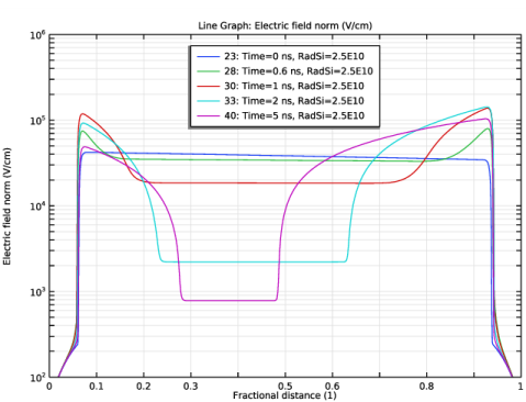
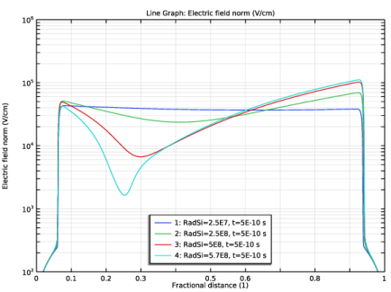
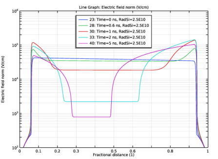
In the Settings window for 1D Plot Group, type Fig. 7C Electric Field Distribution at Several Times in the Label text field.
|
|
3
|
|
4
|
|
5
|
|
6
|
|
1
|
In the Model Builder window, expand the Fig. 7C Electric Field Distribution at Several Times node, then click Line Graph 1.
|
|
2
|
|
3
|
|
4
|
|
5
|
|
1
|
|
2
|
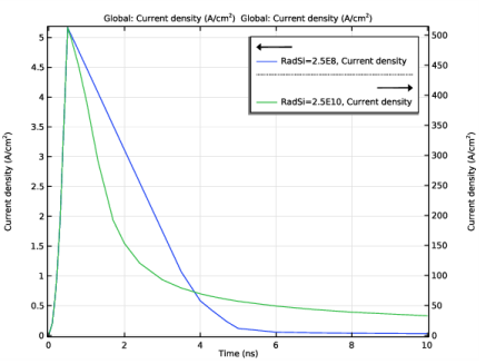
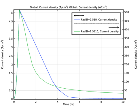
In the Settings window for 1D Plot Group, type Fig. 8 Transient Photocurrent Response in the Label text field.
|
|
3
|
|
4
|
|
1
|
|
2
|
|
3
|
|
4
|
|
5
|
|
6
|
|
7
|
Click to expand the Legends section.
|
|
1
|
|
2
|
|
3
|
|
4
|
|
5
|
|
1
|
|
2
|
|
3
|
|
4
|
|
1
|
|
2
|
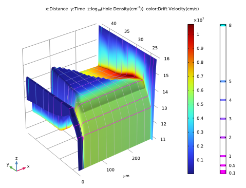
In the Settings window for 2D Plot Group, type Evolution of Hole Density Profile and Drift Velocity in the Label text field.
|
|
3
|
|
4
|
In the Title text area, type x:Distance y:Time z:log<sub>10</sub>(Hole Density(cm<sup>-3</sup>)) color:Drift Velocity(cm/s).
|
|
1
|
|
2
|
|
3
|
|
4
|
|
1
|
|
2
|
|
3
|
|
4
|
|
1
|
|
2
|
|
3
|
|
1
|
In the Model Builder window, right-click Evolution of Hole Density Profile and Drift Velocity and choose Contour.
|
|
2
|
|
3
|
|
4
|
|
5
|
|
6
|
|
7
|
|
1
|
In the Model Builder window, under Results>Evolution of Hole Density Profile and Drift Velocity>Surface 1 click Height Expression 1.
|
|
2
|
|
3
|
|
4
|
Right-click Results>Evolution of Hole Density Profile and Drift Velocity>Surface 1>Height Expression 1 and choose Copy.
|
|
1
|
|
2
|
|
3
|
|
4
|
|
5
|
|
6
|
|
7
|
|
8
|
|
9
|
|
10
|
|
11
|
|
12
|