|
|
|
|
1
|
|
2
|
|
3
|
Click Add.
|
|
4
|
Click
|
|
5
|
|
6
|
Click
|
|
1
|
|
2
|
|
3
|
|
1
|
|
2
|
|
3
|
|
4
|
Browse to the model’s Application Libraries folder and double-click the file double_barrier_1d_param.txt.
|
|
1
|
|
2
|
|
3
|
|
4
|
|
6
|
|
1
|
|
2
|
|
3
|
|
1
|
In the Model Builder window, under Component 1 (comp1)>Schrödinger Equation (schr) click Effective Mass 1.
|
|
2
|
|
3
|
|
1
|
|
2
|
|
3
|
|
1
|
|
3
|
|
4
|
|
1
|
|
3
|
|
4
|
|
1
|
|
2
|
|
3
|
|
1
|
|
2
|
|
3
|
|
1
|
|
2
|
|
3
|
|
4
|
|
5
|
|
6
|
|
1
|
|
2
|
|
3
|
|
4
|
|
1
|
|
2
|
|
3
|
Click
|
|
5
|
|
1
|
In the Model Builder window, under Results click Potential Energy, Eigenenergy, and Wave Function (schr).
|
|
2
|
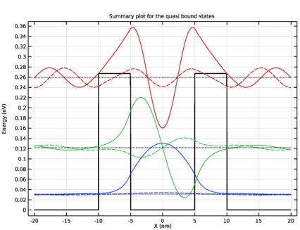
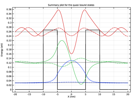
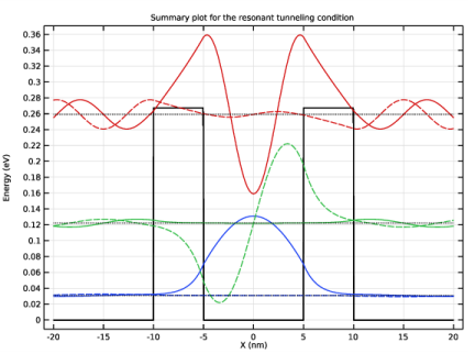
In the Settings window for 1D Plot Group, type Quasi bound state summary plot in the Label text field.
|
|
3
|
|
4
|
|
5
|
|
6
|
|
7
|
|
8
|
|
9
|
|
1
|
|
2
|
|
4
|
Click
|
|
1
|
Go to the Table window.
|
|
1
|
|
2
|
|
3
|
|
4
|
|
5
|
|
1
|
In the Settings window for Time Dependent, click to expand the Values of Dependent Variables section.
|
|
2
|
Find the Initial values of variables solved for subsection. From the Settings list, choose User controlled.
|
|
3
|
|
4
|
|
5
|
In the Settings window for Study, type Study 2 Time evolution of the 3rd quasi bound state in the Label text field.
|
|
1
|
|
2
|
In the Settings window for Initial Values, type Initial Values 2 for time dependent study in the Label text field.
|
|
3
|
|
4
|
|
1
|
In the Model Builder window, under Study 2 Time evolution of the 3rd quasi bound state click Step 1: Time Dependent.
|
|
2
|
|
3
|
|
4
|
|
1
|
|
2
|
|
3
|
|
4
|
|
1
|
|
2
|
|
3
|
|
4
|
|
1
|
|
2
|
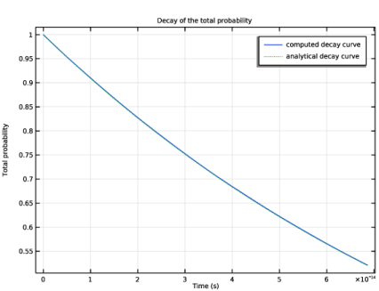
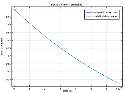
In the Settings window for 1D Plot Group, type Compare decay of total probability in the Label text field.
|
|
3
|
Locate the Data section. From the Dataset list, choose Study 2 Time evolution of the 3rd quasi bound state/Solution 6 (sol6).
|
|
4
|
|
5
|
|
6
|
|
7
|
|
1
|
|
2
|
|
4
|
Click to expand the Coloring and Style section. Find the Line style subsection. From the Line list, choose Cycle.
|
|
5
|
|
1
|
|
2
|
In the Settings window for Open Boundary, type Open Boundary 2 for resonant tunneling study in the Label text field.
|
|
4
|
|
5
|
In the Show More Options dialog box, in the tree, select the check box for the node Physics>Advanced Physics Options.
|
|
6
|
Click OK.
|
|
7
|
|
8
|
|
9
|
From the list, choose Incoming.
|
|
1
|
|
2
|
|
3
|
Find the Studies subsection. In the Select Study tree, select Preset Studies for Selected Physics Interfaces>Eigenvalue.
|
|
4
|
|
5
|
|
1
|
|
2
|
|
3
|
|
4
|
Locate the Physics and Variables Selection section. Select the Modify model configuration for study step check box.
|
|
5
|
In the tree, select Component 1 (comp1)>Schrödinger Equation (schr)>Initial Values 2 for time dependent study.
|
|
6
|
Click
|
|
7
|
|
8
|
|
1
|
|
2
|
|
3
|
|
4
|
|
1
|
|
2
|
|
3
|
Click
|
|
5
|
|
1
|
|
1
|
In the Model Builder window, under Results, Ctrl-click to select Probability Density (schr) 2, Potential Energy (schr) 1, and Effective Mass (schr) 1.
|
|
2
|
Right-click and choose Delete.
|
|
1
|
In the Model Builder window, under Results click Potential Energy, Eigenenergy, and Wave Function (schr).
|
|
2
|
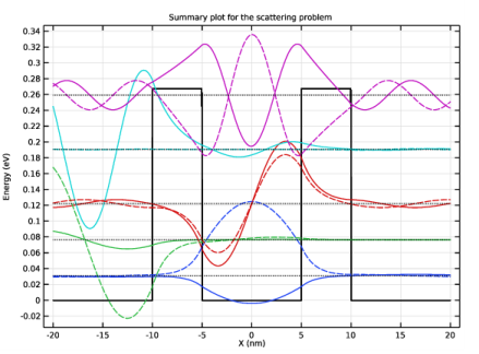
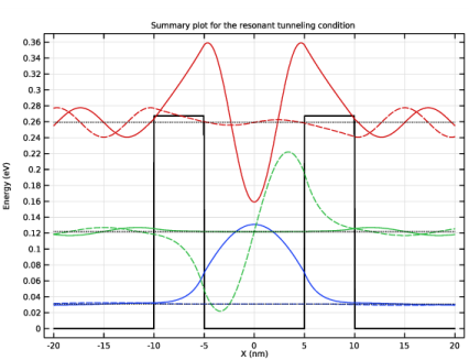
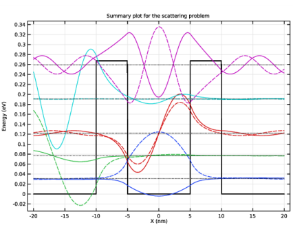
In the Settings window for 1D Plot Group, type Resonant tunneling summary plot in the Label text field.
|
|
3
|
|
4
|
|
5
|
|
6
|
|
7
|
|
8
|
|
9
|
|
1
|
|
2
|
|
4
|
Click
|
|
1
|
Go to the Table window.
|
|
1
|
|
2
|
|
3
|
|
1
|
|
2
|
In the Settings window for Open Boundary, type Open Boundary 3 for transmission vs. energy study in the Label text field.
|
|
4
|
|
5
|
|
1
|
|
2
|
|
3
|
|
4
|
|
5
|
|
1
|
|
2
|
|
3
|
In the tree, select Component 1 (comp1)>Schrödinger Equation (schr)>Initial Values 2 for time dependent study.
|
|
4
|
Click
|
|
5
|
|
6
|
Click
|
|
8
|
|
9
|
|
10
|
|
1
|
|
1
|
In the Model Builder window, under Results, Ctrl-click to select Probability Density (schr) 2, Potential Energy (schr) 1, and Effective Mass (schr) 1.
|
|
2
|
Right-click and choose Delete.
|
|
1
|
In the Model Builder window, under Results click Potential Energy, Energy, and Wave Function (schr).
|
|
2
|
|
3
|
|
4
|
|
5
|
|
6
|
|
7
|
|
8
|
|
9
|
|
10
|
|
11
|
|
1
|
|
2
|
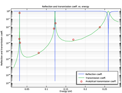
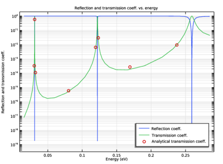
In the Settings window for 1D Plot Group, type Reflection & Transmission vs. Energy in the Label text field.
|
|
3
|
Locate the Data section. From the Dataset list, choose Study 4 Transmission vs. energy/Solution 12 (sol12).
|
|
1
|
|
2
|
|
4
|
|
5
|
|
6
|
|
1
|
|
2
|
|
3
|
|
4
|
|
5
|
|
6
|
|
7
|
Select the y-axis label check box. In the associated text field, type Reflection and transmission coeff..
|
|
8
|
|
1
|
|
2
|
In the Settings window for Table, type Analytical transmission coefficients in the Label text field.
|
|
3
|
|
4
|
Browse to the model’s Application Libraries folder and double-click the file double_barrier_1d_anal.csv.
|
|
5
|
|
1
|
Go to the Table window.
|
|
2
|
|
1
|
In the Model Builder window, under Results>Reflection & Transmission vs. Energy click Table Graph 1.
|
|
2
|
|
3
|
|
4
|
|
5
|
|
6
|
|
1
|
|
2
|
|
3
|
|
4
|
In the tree, select Component 1 (comp1)>Schrödinger Equation (schr)>Initial Values 2 for time dependent study.
|
|
5
|
Click
|
|
6
|
In the tree, select Component 1 (comp1)>Schrödinger Equation (schr)>Open Boundary 2 for resonant tunneling study.
|
|
7
|
Click
|
|
8
|
In the tree, select Component 1 (comp1)>Schrödinger Equation (schr)>Open Boundary 3 for transmission vs. energy study.
|
|
9
|
Click
|
|
1
|
In the Model Builder window, under Study 2 Time evolution of the 3rd quasi bound state click Step 1: Time Dependent.
|
|
2
|
|
3
|
|
4
|
In the tree, select Component 1 (comp1)>Schrödinger Equation (schr)>Open Boundary 2 for resonant tunneling study.
|
|
5
|
Click
|
|
6
|
In the tree, select Component 1 (comp1)>Schrödinger Equation (schr)>Open Boundary 3 for transmission vs. energy study.
|
|
7
|
Click
|
|
1
|
|
2
|
|
3
|
In the tree, select Component 1 (comp1)>Schrödinger Equation (schr)>Open Boundary 3 for transmission vs. energy study.
|
|
4
|
Click
|