PDF

Stability of a Turbocharger Under the Influence of Cross-Coupled Bearing Forces
Introduction
A turbocharger is often supported by hydrodynamic journal bearings. Such bearings naturally have the cross-coupled forces present in them. These cross-coupled forces act as a negative damping in the system. Due to this, near the critical speed, the vibration amplitude in the turbocharger can become large, ultimately leading to the bearing failure. In this example we study the influence of these cross-coupled forces on the dynamics of the rotor.
Variation in the eigenfrequencies and logarithmic decrement with the rotational speed of the rotor gives the idea of the stability state of the overall system. Response of the turbocharger due to external forces at the turbine and compressor is also studied. The waterfall diagram clearly shows that the response amplitude is maximum in the resonance conditions.
Model Definition
The model consists of a turbocharger rotor supported by two bearings, one near the compressor and another near turbine, making both the compressor and turbine overhung on the shaft. The geometry of the rotor is shown in Figure 1.
Figure 1: Rotor geometry.
Two different analyses are performed:
Case 1 — Eigenfrequency Analysis
In this case, eigenfrequency analysis is performed for the different angular speeds of the turbocharger. Structural damping is added to damp the high frequency vibrations of the rotor. The bearings are modeled by equivalent stiffness and damping constants. Bending stiffness and damping in the bearings are neglected.
Properties of the bearings used in this analysis are given in Table 1:
kyy (N/m)
kzz (N/m)
kyz (N/m)
kzy (N/m)
Two cases of the bearing stiffness are considered. In the first, the cross-coupled stiffness kyz and kzy are ignored and in the second all four components of the stiffness are present. The angular speed of the rotor is varied from 0 rpm to 100,000 rpm in steps of 5,000 rpm. The variations in natural frequencies and logarithmic decrements with angular speed of the rotor are analyzed.
CAse2 — Frequency response Analysis
In this case, you analyze the harmonic response of the turbocharger rotor due to the mass eccentricities at both turbine and compressor. The angular speed of the shaft is varied from 2,000 rpm to 100,000 rpm in steps of 2,000 rpm. The frequency is varied from 100 to 3000 Hz in steps of 100 Hz. Variations in the frequency spectrum of the displacement at a point on the rotor is studied.
Results and Discussion
Eigenfrequency analysis
The mode shape of the turbocharger for the fourth mode is shown in Figure 2. In this mode primarily the compressor undergoes the whirl of significant amplitude as compared to the other parts of the rotor. Tilt in both the turbine and the­­­ compressor is also significant.
Figure 2: Mode shape of the turbocharger.
The whirl plot for the sixth mode is shown in Figure 3. In this mode whirling of both compressor and turbine is significant.
Figure 3: Whirl plot.
Campbell plots, shown in Figure 4 and Figure 5, compares the eigenfrequency variation of the rotor excluding and including the cross-coupled stiffness of the bearings, respectively. There is no appreciable change in the eigenfrequency variation due to cross-coupled stiffness except that third and fourth modes frequencies are more closer in the presence of cross-coupled stiffness.
Figure 4: Campbell plot without cross-coupled stiffness.
Figure 5: Campbell plot with cross-coupled stiffness.
The logarithmic decrement is a parameter that gives the stability state of the system. If the logarithmic decrement is positive the response is said to be stable and vice versa. A zero value indicates no damping in that particular mode. The expression for the logarithmic decrement in terms of eigenvalues is:
A plot of the logarithmic decrement as a function of the rotor angular speed is shown in Figure 6 and Figure 7. This plot shows how the damping in a particular mode changes with the angular speed of the rotor. The logarithmic decrement in the absence of cross-coupled stiffness is positive indicating that the natural modes are stable in the absence of cross-coupled bearing stiffness. In the presence of cross-coupled stiffness, many modes have negative logarithmic decrement even at small rotor speeds. This indicates that the presence of cross-coupled stiffness makes the vibrational modes unstable and hence it is dangerous to operate the turbocharger rotor at these speeds.
Figure 6: Logarithmic decrement without cross-coupled stiffness.
Figure 7: Logarithmic decrement with cross-coupled stiffness.
Cross-coupled stiffness in the hydrodynamic bearings can be reduced by changing the bearing design. For example, the tilted pad bearings are known to have the least cross-coupled stiffness. Other way to control the response is to add more damping in the system, for example, using the squeeze film dampers at various locations.
frequency response analysis
The displacement response with cross-coupled stiffness of the turbocharger operating at 100,000 rpm and subjected to a harmonic loading at 3000 Hz is shown in Figure 8.
Figure 8: Displacement response at 3000 Hz.
The waterfall plot for the displacement at the first bearing location is shown in Figure 9 and Figure 10. The waterfall plot shows the variation in the frequency spectrum of the rotor with the change in its angular speed. In the absence of the cross-coupling forces in the bearing (Figure 9) large peaks are observed for certain combinations of the loading frequency and rotor speed. If the cross-coupling forces are present (Figure 10) peaks are more or less uniform.
Figure 9: Waterfall plot without cross-coupled stiffness.
Figure 10: Waterfall plot with cross-coupled stiffness.
Application Library path: Rotordynamics_Module/Automotive_and_Aerospace/turbocharger_stability_analysis
Modeling Instructions
From the File menu, choose New.
New
In the New window, click  Model Wizard.
Model Wizard
1
In the Model Wizard window, click  3D.
2
In the Select Physics tree, select Structural Mechanics>Rotordynamics>Solid Rotor (rotsld).
3
Click Add.
4
Click  Study.
5
In the Select Study tree, select General Studies>Eigenfrequency.
6
Geometry 1
Import 1 (imp1)
Import the turbocharger geometry.
1
In the Home toolbar, click  Import.
2
In the Settings window for Import, locate the Import section.
3
Click  Browse.
4
5
Click  Build All Objects.
Global Definitions
Create the model parameters.
Parameters 1
1
In the Model Builder window, under Global Definitions click Parameters 1.
2
In the Settings window for Parameters, locate the Parameters section.
3
Add Material
1
In the Home toolbar, click  Add Material to open the Add Material window.
2
Go to the Add Material window.
3
In the tree, select Built-in>Structural steel.
4
Click the right end of the Add to Component split button in the window toolbar.
5
From the menu, choose Component 1 (comp1).
6
In the Home toolbar, click  Add Material to close the Add Material window.
Definitions
Create the selection for the compressor and turbine for later use.
Compressor
1
In the Definitions toolbar, click  Explicit.
2
3
In the Settings window for Explicit, type Compressor in the Label text field.
Turbine
1
In the Definitions toolbar, click  Explicit.
2
3
In the Settings window for Explicit, type Turbine in the Label text field.
Solid Rotor (rotsld)
1
In the Model Builder window, under Component 1 (comp1) click Solid Rotor (rotsld).
2
In the Settings window for Solid Rotor, locate the Rotor Speed section.
3
Set the Discretization to Linear to save the computation time. A Quadratic interpolation can be used for better accuracy.
4
Click to expand the Discretization section. From the Displacement field list, choose Linear.
Linear Elastic Material 1
Add the material damping in the shaft.
1
In the Model Builder window, under Component 1 (comp1)>Solid Rotor (rotsld) click Linear Elastic Material 1.
Damping 1
1
In the Physics toolbar, click  Attributes and choose Damping.
2
In the Settings window for Damping, locate the Damping Settings section.
3
In the αdM text field, type 6.04.
4
In the βdK text field, type 2e-6.
First Support 1
1
In the Model Builder window, under Component 1 (comp1)>Solid Rotor (rotsld)>Rotor Axis 1 click First Support 1.
2
Second Support 1
1
In the Model Builder window, click Second Support 1.
2
Fixed Axial Rotation 1
1
In the Model Builder window, under Component 1 (comp1)>Solid Rotor (rotsld) click Fixed Axial Rotation 1.
2
Fixed Axial Rotation 2
1
Right-click Component 1 (comp1)>Solid Rotor (rotsld)>Fixed Axial Rotation 1 and choose Duplicate.
2
Journal Bearing 1
1
In the Physics toolbar, click  Boundaries and choose Journal Bearing.
2
3
In the Settings window for Journal Bearing, locate the Bearing Orientation section.
4
Specify the Orientation vector defining local y direction vector as
5
Locate the Bearing Properties section. From the Bearing model list, choose Total spring and damping constant.
6
In the ku table, enter the following settings:
7
In the kθ table, enter the following settings:
The parameter p is used for enabling and disabling the cross-coupled stiffness.
Journal Bearing 2
1
Right-click Journal Bearing 1 and choose Duplicate.
2
In the Settings window for Journal Bearing, locate the Boundary Selection section.
3
Click  Clear Selection.
4
5
Locate the Bearing Properties section. In the ku table, enter the following settings:
6
In the kθ table, enter the following settings:
Rigid Material: Turbine
1
In the Physics toolbar, click  Domains and choose Rigid Material.
2
In the Settings window for Rigid Material, locate the Domain Selection section.
3
From the Selection list, choose Turbine.
4
In the Label text field, type Rigid Material: Turbine.
Applied Force 1
1
In the Physics toolbar, click  Attributes and choose Applied Force.
2
In the Settings window for Applied Force, locate the Applied Force section.
3
Specify the F vector as
Rigid Material: Compressor
1
In the Model Builder window, right-click Rigid Material: Turbine and choose Duplicate.
2
In the Settings window for Rigid Material, type Rigid Material: Compressor in the Label text field.
3
Locate the Domain Selection section. Click  Clear Selection.
4
Applied Force 1
1
In the Model Builder window, expand the Rigid Material: Compressor node, then click Applied Force 1.
2
In the Settings window for Applied Force, locate the Applied Force section.
3
Specify the F vector as
Mesh 1
Swept 1
1
In the Mesh toolbar, click  Swept.
2
In the Settings window for Swept, locate the Domain Selection section.
3
From the Geometric entity level list, choose Domain.
4
Free Tetrahedral 1
In the Mesh toolbar, click  Free Tetrahedral.
Size 1
1
In the Model Builder window, right-click Swept 1 and choose Size.
2
In the Settings window for Size, locate the Element Size section.
3
From the Predefined list, choose Extra fine.
4
Click  Build All.
Study 1
Parametric Sweep
1
In the Study toolbar, click  Parametric Sweep.
2
In the Settings window for Parametric Sweep, locate the Study Settings section.
3
Click  Add twice.
4
5
From the Sweep type list, choose All combinations.
Step 1: Eigenfrequency
1
In the Model Builder window, click Step 1: Eigenfrequency.
2
In the Settings window for Eigenfrequency, locate the Study Settings section.
3
Select the Desired number of eigenfrequencies check box. In the associated text field, type 9.
4
In the Study toolbar, click  Compute.
Results
Mode Shape (rotsld)
The following instructions will generate the mode shape shown in Figure 2.
1
In the Settings window for 3D Plot Group, locate the Data section.
2
From the Eigenfrequency (Hz) list, choose 2009.5+19.004i.
3
Click the  Go to YZ View button in the Graphics toolbar.
4
Click the  Zoom Extents button in the Graphics toolbar.
5
In the Mode Shape (rotsld) toolbar, click  Plot.
You can select the different eigenfrequencies from the list to analyze the corresponding mode shapes.
Whirl (rotsld)
The following instructions will generate the whirl plot shown in Figure 3.
1
In the Model Builder window, click Whirl (rotsld).
2
In the Settings window for 3D Plot Group, locate the Data section.
3
From the Eigenfrequency (Hz) list, choose 2228.1-306.44i.
Whirl 1
1
In the Model Builder window, expand the Whirl (rotsld) node, then click Whirl 1.
2
In the Settings window for Whirl, locate the Coloring and Style section.
3
In the Number of planes text field, type 1.
4
In the Number of rings text field, type 20.
5
Click  Change Color Table.
6
In the Color Table dialog box, select Thermal>HeatCamera in the tree.
7
8
Click the  Zoom Extents button in the Graphics toolbar.
9
In the Whirl (rotsld) toolbar, click  Plot.
10
The Campbell plots excluding and including the cross coupled stiffness effects are shown in Figure 4 and Figure 5, respectively. Follow the instructions below to reproduce them.
11
In the Home toolbar, click  Add Predefined Plot.
Add Predefined Plot
1
Go to the Add Predefined Plot window.
2
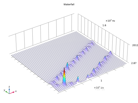
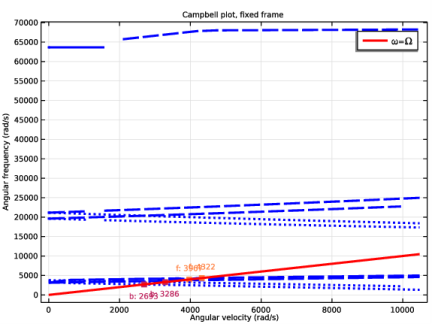
In the tree, select Study 1/Parametric Solutions 1 (sol2)>Solid Rotor>Campbell Plot, Fixed Frame (rotsld).
3
Click Add Plot in the window toolbar.
4
In the Home toolbar, click  Add Predefined Plot.
Results
Campbell Plot, Fixed Frame (rotsld)
1
In the Model Builder window, under Results click Campbell Plot, Fixed Frame (rotsld).
2
In the Settings window for 1D Plot Group, locate the Data section.
3
From the Parameter selection (p) list, choose First.
4
Click the  Zoom Extents button in the Graphics toolbar.
5
In the Campbell Plot, Fixed Frame (rotsld) toolbar, click  Plot.
Switch the parameter p from first to last to analyze the effect of the cross-coupled stiffness.
6
From the Parameter selection (p) list, choose Last.
7
In the Campbell Plot, Fixed Frame (rotsld) toolbar, click  Plot.
Logarithmic Decrement
The following instructions generate the Logarithmic decrement plots shown in Figure 6 and Figure 7.
1
In the Home toolbar, click  Add Plot Group and choose 1D Plot Group.
2
In the Settings window for 1D Plot Group, type Logarithmic Decrement in the Label text field.
3
Locate the Data section. From the Dataset list, choose Study 1/Parametric Solutions 1 (sol2).
4
From the Parameter selection (p) list, choose First.
5
Click to expand the Title section. From the Title type list, choose Label.
6
Click the  Show Legends button in the Graphics toolbar.
Global 1
1
Right-click Logarithmic Decrement and choose Global.
2
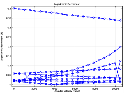
In the Settings window for Global, click Replace Expression in the upper-right corner of the y-Axis Data section. From the menu, choose Component 1 (comp1)>Solid Rotor>Whirl frequencies>rotsld.log_dec - Logarithmic decrement.
3
Locate the x-Axis Data section. From the Axis source data list, choose Outer solutions.
4
From the Parameter list, choose Expression.
5
In the Expression text field, type rotsld.Ovg.
6
Click to expand the Coloring and Style section. Find the Line style subsection. From the Line list, choose Dashed.
7
From the Color list, choose Blue.
8
From the Width list, choose 2.
9
Find the Line markers subsection. From the Marker list, choose Circle.
10
Click the  Zoom Extents button in the Graphics toolbar.
11
In the Logarithmic Decrement toolbar, click  Plot.
Switch the value of the parameter p from First to Last to analyze the effect of cross-coupled stiffness on logarithmic decrement.
Logarithmic Decrement
1
In the Model Builder window, click Logarithmic Decrement.
2
In the Settings window for 1D Plot Group, locate the Data section.
3
From the Parameter selection (p) list, choose Last.
4
Click the  Zoom Extents button in the Graphics toolbar.
5
In the Logarithmic Decrement toolbar, click  Plot.
Animation 1
Finally you can create the animation of the Whirl using the following instructions.
1
In the Results toolbar, click  Animation and choose Player.
2
In the Settings window for Animation, locate the Scene section.
3
From the Subject list, choose Whirl (rotsld).
4
Locate the Animation Editing section. From the Sequence type list, choose Dynamic data extension.
5
Click the  Play button in the Graphics toolbar.
Root
Eigenfrequency Analysis is finished now. Now you will analyze the harmonic response of the turbocharger due to external forces on turbine and compressor.
Add Study
1
In the Home toolbar, click  Add Study to open the Add Study window.
2
Go to the Add Study window.
3
Find the Studies subsection. In the Select Study tree, select General Studies>Frequency Domain.
4
Click Add Study in the window toolbar.
5
In the Home toolbar, click  Add Study to close the Add Study window.
Study 2
Step 1: Frequency Domain
1
In the Settings window for Frequency Domain, locate the Study Settings section.
2
In the Frequencies text field, type range(100,100,3000).
3
In the Home toolbar, click Desktop Layout and choose Reset Desktop.
Parametric Sweep
1
In the Study toolbar, click  Parametric Sweep.
2
In the Settings window for Parametric Sweep, locate the Study Settings section.
3
Click  Add twice.
4
5
From the Sweep type list, choose All combinations.
6
In the Study toolbar, click  Compute.
Results
Displacement (rotsld)
The first default plot for Study 2 is a stress plot, which is only meaningful in an elastic domain. Change this plot to show the displacement response as in Figure 8 using the following instructions.
1
In the Settings window for 3D Plot Group, type Displacement (rotsld) in the Label text field.
Surface
1
In the Model Builder window, expand the Displacement (rotsld) node, then click Surface.
2
In the Settings window for Surface, locate the Expression section.
3
In the Expression text field, type rotsld.disp.
4
Locate the Coloring and Style section. Click  Change Color Table.
5
In the Color Table dialog box, select Rainbow>Prism in the tree.
6
7
In the Displacement (rotsld) toolbar, click  Plot.
Displacement (rotsld)
1
Click the  Zoom Extents button in the Graphics toolbar.
2
In the Model Builder window, click Displacement (rotsld).
3
In the Displacement (rotsld) toolbar, click  Plot.
Cut Point 3D 1
The following instructions generate the Waterfall plots shown in Figure 9 and Figure 10. To do that we start by creating a Cut Point at the center of the compressor end of the shaft.
1
In the Results toolbar, click  Cut Point 3D.
2
In the Settings window for Cut Point 3D, locate the Point Data section.
3
In the X text field, type 0.
4
In the Y text field, type 0.0624.
5
In the Z text field, type 0.
6
Locate the Data section. From the Dataset list, choose Study 2/Parametric Solutions 2 (sol46).
Waterfall plot
1
In the Results toolbar, click  3D Plot Group.
2
In the Settings window for 3D Plot Group, locate the Data section.
3
From the Dataset list, choose Cut Point 3D 1.
4
In the Label text field, type Waterfall plot.
Waterfall 1
1
In the Waterfall plot toolbar, click  More Plots and choose Waterfall.
2
In the Settings window for Waterfall, locate the Data section.
3
From the Dataset list, choose Cut Point 3D 1.
4
From the Parameter selection (p) list, choose First.
5
Locate the Expression section. In the Expression text field, type abs(u).
6
Locate the x-Axis Data section. In the Expression text field, type Ow.
7
Locate the y-Axis Data section. In the Expression text field, type freq.
8
Locate the Coloring and Style section. Click  Change Color Table.
9
In the Color Table dialog box, select Rainbow>Prism in the tree.
10
11
Click the  Zoom Extents button in the Graphics toolbar.
12
In the Waterfall plot toolbar, click  Plot.
13
Click the  Scene Light button in the Graphics toolbar.
Adjust the grids in the View corresponding to the Waterfall Plot.
14
In the Model Builder window, expand the Results>Views node.
Camera
1
In the Model Builder window, expand the Results>Views>View 3D 3 node, then click Camera.
2
In the Settings window for Camera, locate the Grid section.
3
Select the Manual spacing check box.
4
In the x spacing text field, type 200.
5
In the y spacing text field, type 200.
6
In the z spacing text field, type 2.
7
Click  Update.
Waterfall 1
1
Click the  Zoom Extents button in the Graphics toolbar.
2
In the Model Builder window, under Results>Waterfall plot click Waterfall 1.
3
In the Settings window for Waterfall, locate the Data section.
4
From the Parameter selection (p) list, choose Last.
5
In the Waterfall plot toolbar, click  Plot.
Animation 1
Finally use the following instructions to create the animation of the Displacement response.
Animation 2
1
In the Model Builder window, under Results>Export right-click Animation 1 and choose Duplicate.
2
In the Settings window for Animation, locate the Scene section.
3
From the Subject list, choose Displacement (rotsld).
4
Click the  Play button in the Graphics toolbar.