PDF

Whirling of Uniform Shaft Under Gravity
Introduction
In this model, you analyze the dynamics of a rotating shaft under gravity and supported by two hydrodynamic bearings at its ends. Coupling between the rotor and the bearings is achieved through the Beam Rotor with Hydrodynamics Bearing multiphysics interface in the Rotordynamics Module.
Model Definition
The rotor is modeled as a beam of length L and diameter D. The material parameters of the rotor are listed in Table 1.
The rotor rotates inside the bearings with an angular speed Ω .
The bearing rotor assembly is shown in Figure 1 below.
Figure 1: Rotor configuration.
This simulation considers a plain bearing. The parameters needed for the fluid-film simulation are the dynamic viscosity, the density at cavitation pressure, and the compressibility. The values of the parameters are summarized in Table 2 below.
10-7 Pa-1
Results and Discussion
Figure 2 below shows the stress profile on the rotor with the maximum bending stress in the middle part.
Figure 2: Rotor stress profile.
A plot of the bearing fluid pressure is shown in Figure 3.
Figure 3: Fluid pressure.
The orbit of the journal in the yz-plane at 0 is shown in Figure 4. Initially, the journal is at the center of the bearing and is subjected to gravitational acceleration. As the journal moves in the bearing, the pressure profile of the fluid film changes, which resists the motion of the journal. Therefore, due to the inertia, the lateral displacement of the middle part of the rotor is larger than that of the journal in the bearing, resulting in the bending of the rotor. Because the rotor is also rotating about its own axis, it experiences a gyroscopic moment due to the bending of the rotor. The gyroscopic moment causes the rotor to whirl about its initial axis. Hence, the journal spirals out and eventually reaches a steady orbit.
Figure 4: Journal orbit.
A plot of the y and z components of the acceleration of the journal is shown in Figure 5. The acceleration reaches a steady value around the time t = 0.1 s.
Figure 5: Acceleration vs. time.
Figure 6 shows the frequency spectrum for the acceleration signal displayed in Figure 5. For both the y and components of the acceleration, the spectrum contains one dominating frequency around 65 Hz which is approximately 0.43 times the rotational frequency of the rotor. This type of whirling is often categorized as a half-frequency whirl.
Contributions of other frequencies are small except for the one around 130 Hz. This produces some perturbations of the acceleration curve, as can be observed by the wiggles in Figure 5.
Figure 6: Frequency spectrum of acceleration.
Application Library path: Rotordynamics_Module/Tutorials/rotor_whirl
Modeling Instructions
From the File menu, choose New.
New
In the New window, click  Model Wizard.
Model Wizard
1
In the Model Wizard window, click  3D.
2
In the Select Physics tree, select Structural Mechanics>Rotordynamics>Beam Rotor with Hydrodynamic Bearing.
3
Click Add.
4
Click  Study.
5
In the Select Study tree, select General Studies>Time Dependent.
6
Global Definitions
Parameters 1
1
In the Model Builder window, under Global Definitions click Parameters 1.
2
In the Settings window for Parameters, locate the Parameters section.
3
Geometry 1
Polygon 1 (pol1)
1
In the Geometry toolbar, click  More Primitives and choose Polygon.
2
In the Settings window for Polygon, locate the Coordinates section.
3
From the Data source list, choose Vectors.
4
In the x text field, type 0 L.
5
In the y text field, type 0.
6
In the z text field, type 0.
Now you create plain surfaces at the ends of the rotor to represent bearing.
Cylinder 1 (cyl1)
1
In the Geometry toolbar, click  Cylinder.
2
In the Settings window for Cylinder, locate the Object Type section.
3
From the Type list, choose Surface.
4
Locate the Size and Shape section. In the Radius text field, type D/2.
5
In the Height text field, type Lj.
6
Locate the Axis section. From the Axis type list, choose x-axis.
Cylinder 2 (cyl2)
1
Right-click Cylinder 1 (cyl1) and choose Duplicate.
2
In the Settings window for Cylinder, locate the Position section.
3
In the x text field, type L-Lj.
4
Click  Build All Objects.
5
Click the  Zoom Extents button in the Graphics toolbar.
Materials
Material 1 (mat1)
1
In the Model Builder window, under Component 1 (comp1) right-click Materials and choose Blank Material.
2
In the Settings window for Material, locate the Geometric Entity Selection section.
3
From the Geometric entity level list, choose Edge.
4
From the Selection list, choose All edges.
5
In the Model Builder window, expand the Material 1 (mat1) node, then click Basic (def).
6
In the Settings window for Basic, locate the Output Properties section.
7
Click  Select Quantity.
8
In the Physical Quantity dialog box, type density in the text field.
9
Click  Filter.
10
In the tree, select General>Density (kg/m^3).
11
12
In the Settings window for Basic, locate the Output Properties section.
13
Click  Select Quantity.
14
In the Physical Quantity dialog box, type poissonsratio in the text field.
15
Click  Filter.
16
In the tree, select Solid Mechanics>Poisson’s ratio (1).
17
18
In the Settings window for Basic, locate the Output Properties section.
19
Click  Select Quantity.
20
In the Physical Quantity dialog box, type youngsmodulus in the text field.
21
Click  Filter.
22
In the tree, select Solid Mechanics>Young’s modulus (Pa).
23
24
In the Settings window for Basic, locate the Output Properties section.
25
Beam Rotor (rotbm)
1
In the Model Builder window, under Component 1 (comp1) click Beam Rotor (rotbm).
2
In the Settings window for Beam Rotor, locate the Edge Selection section.
3
Click  Clear Selection.
4
5
Locate the Rotor Speed section. In the text field, type Ow.
Rotor Cross Section 1
1
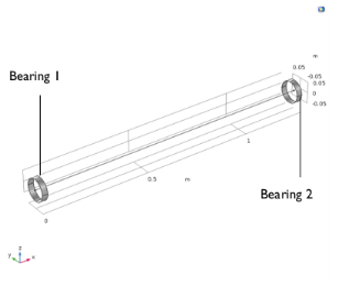
In the Model Builder window, under Component 1 (comp1)>Beam Rotor (rotbm) click Rotor Cross Section 1.
2
In the Settings window for Rotor Cross Section, locate the Cross-Section Definition section.
3
In the do text field, type D.
Gravity 1
1
In the Physics toolbar, click  Edges and choose Gravity.
2
Click the  Show More Options button in the Model Builder toolbar.
3
In the Show More Options dialog box, in the tree, select the check box for the node Physics>Advanced Physics Options.
4
Enable the Advanced Physics Option to add a cavitation to the model.
Hydrodynamic Bearing (hdb)
1
In the Settings window for Hydrodynamic Bearing, locate the Physical Model section.
2
From the Fluid type list, choose Liquid with cavitation.
You can change the compressibility β inside the bearing node.
Hydrodynamic Journal Bearing 1
1
In the Model Builder window, under Component 1 (comp1)>Hydrodynamic Bearing (hdb) click Hydrodynamic Journal Bearing 1.
2
In the Settings window for Hydrodynamic Journal Bearing, locate the Bearing Properties section.
3
In the C text field, type C.
4
Locate the Fluid Properties section. From the μ list, choose User defined. In the associated text field, type mu0.
You need to change the default mesh using the following sequence of commands. This is needed for the accurate coupling between rotor and bearing.
Mesh 1
Beam Rotor
1
In the Mesh toolbar, click  Boundary and choose Edge.
2
In the Settings window for Edge, type Beam Rotor in the Label text field.
3
Distribution 1
1
Right-click Beam Rotor and choose Distribution.
2
In the Settings window for Distribution, locate the Distribution section.
3
In the Number of elements text field, type 150.
Bearing
1
In the Mesh toolbar, click  Boundary and choose Mapped.
2
In the Settings window for Mapped, type Bearing in the Label text field.
3
Click in the Graphics window and then press Ctrl+A to select all boundaries.
Distribution 1
1
Right-click Bearing and choose Distribution.
2
3
In the Settings window for Distribution, locate the Distribution section.
4
In the Number of elements text field, type 20.
Distribution 2
1
In the Model Builder window, right-click Bearing and choose Distribution.
2
3
In the Settings window for Distribution, locate the Distribution section.
4
In the Number of elements text field, type 3.
5
Click  Build All.
Study 1
Step 1: Time Dependent
1
In the Model Builder window, under Study 1 click Step 1: Time Dependent.
2
In the Settings window for Time Dependent, locate the Study Settings section.
3
In the Output times text field, type range(0,5e-4,0.2).
Solution 1 (sol1)
You need to change the default scaling of the dependent variable pfilm.
1
In the Study toolbar, click  Show Default Solver.
2
In the Model Builder window, expand the Solution 1 (sol1) node.
3
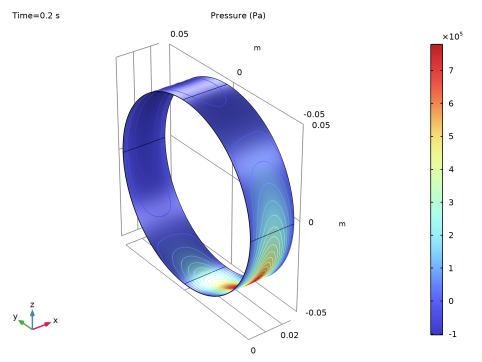
In the Model Builder window, expand the Study 1>Solver Configurations>Solution 1 (sol1)>Dependent Variables 1 node, then click Pressure (comp1.pfilm).
4
In the Settings window for Field, locate the Scaling section.
5
In the Scale text field, type 1.0e5.
Set the Jacobian update of the nonlinear solver to Minimal to reduce the computation time.
6
In the Model Builder window, expand the Study 1>Solver Configurations>Solution 1 (sol1)>Time-Dependent Solver 1 node, then click Fully Coupled 1.
7
In the Settings window for Fully Coupled, click to expand the Method and Termination section.
8
From the Jacobian update list, choose Minimal.
Step 1: Time Dependent
In the Study toolbar, click  Compute.
Results
Stress (rotbm)
The default plots Figure 2 and Figure 3 show rotor stress and fluid pressure respectively.
1
In the Settings window for 3D Plot Group, click to expand the Title section.
2
From the Title type list, choose Manual.
3
In the Title text area, type von Mises stress (N/m<sup>2</sup>).
4
Click the  Zoom Extents button in the Graphics toolbar.
Study 1/Solution 1 (sol1)
Duplicate the solution and select only one bearing to display the fluid pressure on it.
Study 1/Solution 1 (2) (sol1)
1
In the Model Builder window, expand the Results>Datasets node.
2
Right-click Results>Datasets>Study 1/Solution 1 (sol1) and choose Duplicate.
Selection
1
In the Results toolbar, click  Attributes and choose Selection.
2
In the Settings window for Selection, locate the Geometric Entity Selection section.
3
From the Geometric entity level list, choose Boundary.
4
Fluid Pressure (hdb)
1
In the Model Builder window, under Results click Fluid Pressure (hdb).
2
In the Settings window for 3D Plot Group, locate the Data section.
3
From the Dataset list, choose Study 1/Solution 1 (2) (sol1).
4
Locate the Title section. From the Title type list, choose Manual.
5
In the Title text area, type Pressure (Pa) .
6
Locate the Plot Settings section. From the View list, choose New view.
7
In the Fluid Pressure (hdb) toolbar, click  Plot.
8
Click the  Zoom Extents button in the Graphics toolbar.
Orbit
Follow the instructions below to plot the yz-plane orbit of the journal at bearing as shown in Figure 4.
1
In the Model Builder window, expand the Fluid Pressure (hdb) node.
2
Right-click Results and choose 1D Plot Group.
3
In the Settings window for 1D Plot Group, type Orbit in the Label text field.
Point Graph 1
1
Right-click Orbit and choose Point Graph.
2
3
In the Settings window for Point Graph, locate the y-Axis Data section.
4
In the Expression text field, type w/C.
5
Locate the x-Axis Data section. From the Parameter list, choose Expression.
6
In the Expression text field, type v/C.
7
Click to expand the Coloring and Style section. From the Color list, choose Magenta.
Orbit
1
In the Model Builder window, click Orbit.
2
In the Settings window for 1D Plot Group, click to expand the Title section.
3
From the Title type list, choose Manual.
4
In the Title text area, type Orbit of the journal at the left bearing.
5
Locate the Axis section. Select the Preserve aspect ratio check box.
6
In the Orbit toolbar, click  Plot.
7
Click the  Zoom Extents button in the Graphics toolbar.
Use the following instructions to plot the y and z acceleration versus time as shown in Figure 5.
Acceleration vs. Time
1
In the Home toolbar, click  Add Plot Group and choose 1D Plot Group.
2
In the Settings window for 1D Plot Group, type Acceleration vs. Time in the Label text field.
y Acceleration
1
Right-click Acceleration vs. Time and choose Point Graph.
2
In the Settings window for Point Graph, type y Acceleration in the Label text field.
3
4
Locate the y-Axis Data section. In the Expression text field, type vtt.
5
Click to expand the Title section. From the Title type list, choose Manual.
6
Locate the Coloring and Style section. From the Width list, choose 3.
7
Click to expand the Legends section. From the Legends list, choose Manual.
8
Select the Show legends check box.
9
z Acceleration
1
Right-click y Acceleration and choose Duplicate.
2
In the Settings window for Point Graph, type z Acceleration in the Label text field.
3
Locate the y-Axis Data section. In the Expression text field, type wtt.
4
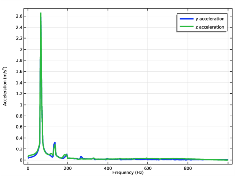
Locate the Legends section. In the table, enter the following settings:
Acceleration vs. Time
1
In the Model Builder window, click Acceleration vs. Time.
2
In the Settings window for 1D Plot Group, locate the Plot Settings section.
3
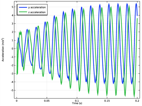
Select the y-axis label check box. In the associated text field, type Acceleration (m/s<sup>2</sup>).
4
Locate the Legend section. From the Position list, choose Upper left.
5
In the Acceleration vs. Time toolbar, click  Plot.
6
Click the  Zoom Extents button in the Graphics toolbar.
Finally plot the frequency component of y and z acceleration as shown in Figure 6.
Acceleration Spectrum
1
Right-click Acceleration vs. Time and choose Duplicate.
2
In the Settings window for 1D Plot Group, type Acceleration Spectrum in the Label text field.
3
Locate the Plot Settings section.
4
Select the x-axis label check box. In the associated text field, type Frequency (Hz).
5
Locate the Legend section. From the Position list, choose Upper right.
y Acceleration
1
In the Model Builder window, expand the Acceleration Spectrum node, then click y Acceleration.
2
In the Settings window for Point Graph, locate the x-Axis Data section.
3
From the Parameter list, choose Discrete Fourier transform.
4
From the Show list, choose Frequency spectrum.
5
From the Scale list, choose Divide by number of frequencies.
z Acceleration
1
In the Model Builder window, click z Acceleration.
2
In the Settings window for Point Graph, locate the x-Axis Data section.
3
From the Parameter list, choose Discrete Fourier transform.
4
From the Show list, choose Frequency spectrum.
5
From the Scale list, choose Divide by number of frequencies.
6
In the Acceleration Spectrum toolbar, click  Plot.
7
Click the  Zoom Extents button in the Graphics toolbar.