|
|
|
|
2·106 N/m
|
|
•
|
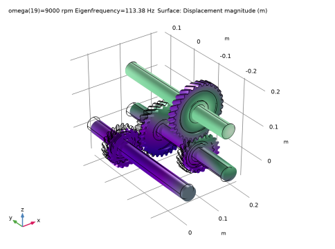
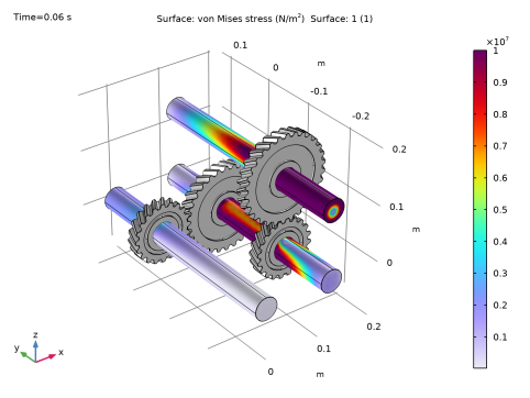
In the time dependent analysis, a resisting load torque of 102 Nm is applied at the opposite end of the driven shaft.
|
|
1
|
|
2
|
|
3
|
Click Add.
|
|
4
|
Click
|
|
5
|
|
6
|
Click
|
|
1
|
|
2
|
|
3
|
|
4
|
Browse to the model’s Application Libraries folder and double-click the file geared_rotors_parameters.txt.
|
|
1
|
|
2
|
|
3
|
|
4
|
|
5
|
|
1
|
|
2
|
|
3
|
Click
|
|
4
|
Browse to the model’s Application Libraries folder and double-click the file geared_rotors.mphbin.
|
|
5
|
Click
|
|
1
|
|
2
|
|
3
|
|
4
|
|
5
|
|
1
|
|
2
|
|
3
|
|
4
|
|
5
|
|
1
|
|
2
|
|
3
|
In the text field, type omega.
|
|
1
|
|
2
|
|
3
|
|
4
|
|
5
|
Click OK.
|
|
1
|
|
2
|
|
3
|
|
4
|
|
5
|
Click OK.
|
|
1
|
|
1
|
|
2
|
|
3
|
|
4
|
|
5
|
Click OK.
|
|
1
|
|
2
|
|
3
|
|
4
|
|
5
|
Click OK.
|
|
1
|
|
1
|
|
2
|
|
3
|
|
4
|
|
5
|
Click OK.
|
|
1
|
|
2
|
|
3
|
|
4
|
|
5
|
Click OK.
|
|
1
|
|
3
|
|
4
|
In the text field, type -omega/gr.
|
|
1
|
|
3
|
|
4
|
In the text field, type omega/gr^2.
|
|
1
|
|
3
|
|
4
|
|
5
|
|
6
|
Click OK.
|
|
7
|
|
8
|
|
1
|
|
3
|
|
4
|
|
5
|
|
6
|
|
7
|
|
8
|
|
9
|
|
1
|
In the Model Builder window, expand the Helical Gear 1 node, then click Center of Rotation: Point 1.
|
|
2
|
|
3
|
|
4
|
|
5
|
Click OK.
|
|
1
|
In the Model Builder window, under Component 1 (comp1)>Solid Rotor (rotsld) right-click Helical Gear 1 and choose Duplicate.
|
|
2
|
|
3
|
|
5
|
|
6
|
|
7
|
|
1
|
In the Model Builder window, expand the Helical Gear 2 node, then click Center of Rotation: Point 1.
|
|
2
|
|
3
|
|
4
|
|
5
|
|
6
|
Click OK.
|
|
1
|
In the Model Builder window, under Component 1 (comp1)>Solid Rotor (rotsld) right-click Helical Gear 1 and choose Duplicate.
|
|
2
|
|
3
|
|
1
|
In the Model Builder window, expand the Helical Gear 3 node, then click Center of Rotation: Point 1.
|
|
2
|
|
3
|
|
4
|
|
5
|
|
6
|
Click OK.
|
|
1
|
In the Model Builder window, under Component 1 (comp1)>Solid Rotor (rotsld) right-click Helical Gear 2 and choose Duplicate.
|
|
2
|
|
3
|
|
1
|
In the Model Builder window, expand the Helical Gear 4 node, then click Center of Rotation: Point 1.
|
|
2
|
|
3
|
|
4
|
|
5
|
|
6
|
Click OK.
|
|
1
|
|
2
|
|
3
|
|
4
|
|
5
|
|
1
|
|
2
|
|
3
|
|
4
|
|
1
|
|
2
|
|
3
|
|
4
|
|
5
|
|
1
|
|
2
|
|
3
|
|
4
|
|
1
|
|
3
|
|
4
|
Specify the Orientation vector defining local y direction vector as
|
|
5
|
Locate the Bearing Properties section. From the Bearing model list, choose Total spring and damping constant.
|
|
6
|
|
1
|
|
2
|
|
3
|
|
5
|
|
1
|
|
2
|
|
3
|
|
5
|
|
1
|
|
2
|
|
3
|
|
5
|
|
1
|
|
2
|
|
3
|
|
1
|
|
2
|
|
3
|
|
5
|
|
1
|
|
3
|
|
4
|
|
1
|
|
2
|
|
3
|
|
4
|
|
1
|
|
2
|
|
1
|
|
2
|
|
3
|
Click
|
|
1
|
|
2
|
|
3
|
|
4
|
|
1
|
|
2
|
|
3
|
|
4
|
|
5
|
|
1
|
|
2
|
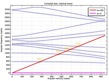
In the tree, select Study 1: Eigenfrequency/Parametric Solutions 1 (sol2)>Solid Rotor>Campbell Plot, Rotating Frame (rotsld).
|
|
3
|
|
4
|
|
1
|
|
2
|
|
1
|
In the Model Builder window, under Results>Campbell Plot, Rotating Frame (rotsld) click Forward Whirl Mode.
|
|
2
|
|
1
|
|
2
|
|
3
|
|
4
|
|
5
|
|
6
|
|
7
|
|
8
|
Clear the Prefix text field.
|
|
9
|
|
10
|
|
11
|
Click Define custom colors.
|
|
13
|
Click Add to custom colors.
|
|
14
|
|
1
|
|
2
|
|
3
|
|
1
|
|
2
|
|
3
|
|
4
|
|
5
|
|
1
|
|
2
|
|
3
|
|
1
|
|
2
|
|
3
|
Click
|
|
1
|
|
2
|
|
3
|
|
4
|
Locate the Physics and Variables Selection section. Select the Modify model configuration for study step check box.
|
|
5
|
|
6
|
Click
|
|
7
|
|
1
|
|
2
|
|
3
|
|
1
|
|
2
|
|
4
|
|
5
|
|
6
|
|
7
|
|
8
|
Click to expand the Coloring and Style section. Find the Line style subsection. From the Line list, choose Cycle.
|
|
9
|
|
10
|
|
1
|
|
2
|
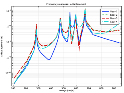
In the Settings window for 1D Plot Group, type Frequency response: x-displacement in the Label text field.
|
|
3
|
|
4
|
|
5
|
|
6
|
|
7
|
|
8
|
|
1
|
In the Model Builder window, expand the Frequency response: x-displacement 1 node, then click Global 1.
|
|
2
|
|
1
|
|
2
|
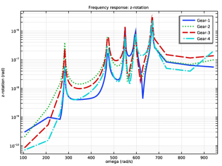
In the Settings window for 1D Plot Group, type Frequency response: z-rotation in the Label text field.
|
|
3
|
|
4
|
|
5
|
|
1
|
|
2
|
|
3
|
|
4
|
|
5
|
|
1
|
|
2
|
|
1
|
|
2
|
|
3
|
|
1
|
|
2
|
|
3
|
In the Model Builder window, expand the Study 3: Time Dependent>Solver Configurations>Solution 110 (sol110)>Time-Dependent Solver 1 node, then click Fully Coupled 1.
|
|
4
|
|
5
|
|
6
|
|
1
|
|
2
|
|
1
|
|
2
|
|
3
|
|
1
|
|
2
|
In the Settings window for Deformation, click Replace Expression in the upper-right corner of the Expression section. From the menu, choose Component 1 (comp1)>Solid Rotor>Displacement>rotsld.us_fix,...,rotsld.ws_fix - Displacement field, fixed frame.
|
|
3
|
Locate the Scale section.
|
|
4
|
|
1
|
|
2
|
|
3
|
|
4
|
|
5
|
|
6
|
|
1
|
|
2
|
|
3
|
|
4
|
|
5
|
|
6
|
|
1
|
|
2
|
|
3
|
|
4
|
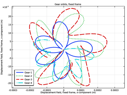
Locate the Point Data section. In the X text field, type rotsld.hlg1.xcx, rotsld.hlg2.xcx, rotsld.hlg3.xcx, rotsld.hlg4.xcx.
|
|
5
|
|
6
|
|
1
|
|
2
|
|
3
|
|
1
|
|
2
|
|
3
|
|
4
|
|
5
|
|
6
|
Click to expand the Coloring and Style section. Find the Line style subsection. From the Line list, choose Cycle.
|
|
7
|
|
8
|
|
9
|
|
1
|
|
2
|
|
3
|
|
4
|
|
5
|
|
6
|
|
7
|
|
1
|
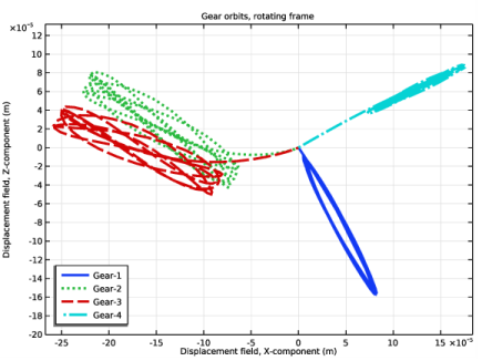
In the Model Builder window, expand the Gear orbits, rotating frame 1 node, then click Point Graph 1.
|
|
2
|
|
3
|
|
4
|
|
1
|
|
2
|
|
3
|
|
4
|
|
1
|
|
2
|
|
3
|
|
1
|
|
2
|
|
4
|
Locate the Coloring and Style section. Find the Line style subsection. From the Line list, choose Cycle.
|
|
5
|
|
6
|
|
1
|
|
2
|
|
3
|
|
4
|
|
5
|
|
6
|
|
7
|
|
1
|
|
2
|
|
3
|
|
4
|
|
5
|
|
6
|
|
7
|
|
1
|
|
2
|
|
3
|
|
1
|
|
2
|
|
3
|
|
4
|
Locate the Coloring and Style section. Find the Line style subsection. From the Line list, choose Cycle.
|
|
5
|
|
6
|
|
7
|
|
1
|
|
2
|
|
3
|
|
4
|
Locate the Legends section. In the table, enter the following settings:
|
|
1
|
|
2
|
|
3
|
|
4
|
|
5
|
|
6
|
|
7
|
|
8
|
|
1
|
|
2
|
|
3
|
|
4
|