You are viewing the documentation for an older COMSOL version. The latest version is available here.
PDF

Shaft Vibration due to Gear Rattle and Bearing Misalignment
Introduction
In a gearbox, vibrations due to gear rattling and bearing misalignment are well known sources of noise. In this example, two shafts connected through a pair of gears are considered. The shafts are supported on roller bearings at their ends. Initially, the driven shaft is unloaded and the driver shaft rotates with a varying speed. Due to backlash, intermittent tooth meshing causes vibrations in the shafts. After some time, a resisting torque is applied to the driven shaft, making the tooth meshing smooth. In order to analyze the effect of bearing misalignment on rotor vibrations, a time-dependent analysis is performed for two cases. In the first case, all bearings are aligned with the shafts, and in the second, one of the bearings (number 2) has a small angular misalignment.
Note: This model requires the Multibody Dynamics Module and the Rotordynamics Module.
Model Definition
The model consists of two shafts connected through a pair of spur gears. The spur gear of the first (driver) shaft transfers rotation to the larger spur gear of the second (driven) shaft. Both shafts are supported at their ends using roller bearings.
The geometry is shown in Figure 1 below.
Figure 1: System geometry.
Shafts
The shafts are made of structural steel, with diameter and length of 20 mm and 300 mm, respectively. The mean angular speed of the driver shaft is assumed to be ω0 = 20 rad/s. It fluctuates about this mean speed as:
Bearings
Each shaft is supported by deep groove ball bearings at the ends. The bearings have the same dimensions and material properties. The properties are given in Table 1.
Gears
The properties of the spur gears are given in Table 2.
The density of the gears, used to compute inertial properties, is equal to the shaft density.
constraints and loads
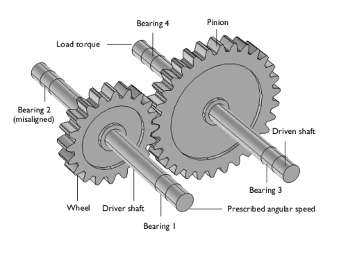
A resisting load torque of 100 Nm is applied at the opposite end of the driven shaft. The torque is activated only after the driver shaft has completed a 45° rotation.
Results and Discussion
Figure 2 shows the axial stress variation in the shafts. In addition to the torque, there are mainly two forces acting on the shafts. One, a gear mesh force acting in the pressure angle direction which bends the shafts in opposite direction and other the reaction forces from the bearing. Reaction forces in the bearing mainly support the shaft against the gear mesh force. Moreover, due to the angular misalignment in one of the bearings, an additional reaction moment is also present to overcome the misalignment in that bearing. The net axial stress in the shaft will be a combination of the bending of the shaft about two axes, one perpendicular to the pressure angle direction, and the other parallel to the misalignment axis. From the stress distribution in the shafts it is clear that the bending in the shaft due to gear mesh force is larger as compared to the bending due to the bearing misalignment. The bearing force direction on the shafts confirms that gear meshing forces are directly transmitted to the bearings in the pressure angle direction.
Figure 2: Stresses and bearing forces.
Figure 3 shows a comparison of angular speeds of the wheel and the pinion, for the cases of an aligned and a misaligned bearing. There is a slightly higher torsional vibration for the case of a misaligned bearing. The rattling vibrations in the misaligned case also persist for longer duration.
Figure 3: Angular velocity of the shafts for aligned bearings (left), and for a misaligned bearing (right).
The axial vibration at the wheel, after the rattling subsides, is shown in Figure 4. In the case of a misaligned bearing, axial vibrations (accelerations) are mainly due to the misalignment in the bearing. As can be seen in Figure 4 that the accelerations for the case of a misaligned bearing are significantly higher than that with aligned bearings.
Due to the angular misalignment in the bearings the force transmitted through the roller to the respective races has an axial component. This is the reason for the significant axial vibration of the shafts with misaligned bearing.
Figure 4: Axial acceleration at the wheel, for aligned bearings (left), and for a misaligned bearing (right).
Frequency spectra for axial vibrations are shown in Figure 5. Compared to the case of aligned bearings, the case of a misaligned bearing shows participation from a broader range of frequencies. Vibration amplitude at higher frequencies are significantly higher in misaligned case.
Figure 5: Frequency spectrum of the axial acceleration at the wheel, for the aligned (left) and misaligned (right) bearing.
Figure 6 shows the bearing force components for bearing 2. The case where the bearing is aligned is shown on the left, and the case where it is misaligned, on the right. In the misaligned case the force variations are slightly larger and contain higher frequencies.
Figure 6: Force in bearing 2, for the aligned (left) and misaligned (right) bearing.
Figure 7 compares the moments in bearing 2. The result for the aligned bearings is presented on the left, and for the misaligned bearing on the right. One can clearly see a large moment about the x-axis in the misaligned case. The moment about z-axis also has slightly higher amplitude variation in misaligned case.
Figure 7: Moments in bearing 2, for the aligned (left) and misaligned (right) bearing.
A comparison of the rotor tilting in bearing 2 is shown in Figure 8 with results for the aligned case on the left and for the misaligned case on the right. Since the misalignment is quite small, the mean titling and amplitude do not differ significantly in both cases. However, in the misaligned case, there is a high frequency variation in the tilting.
Figure 8: Rotor tilting in bearing 2, for the aligned (left) and misaligned (right) bearing.
The gear mesh contact force for the cases of aligned and misaligned bearings are shown in Figure 9. During the rattling vibration, intermittent contact in the gear meshing is clearly visible. The contact force variation is only lightly influenced by the misalignment in the bearing, however, after the shaft loading, rattling persists for longer in the case when bearing is misaligned.
Figure 9: Gear mesh contact forces, for aligned bearings (left), and for a misaligned bearing (right).
Application Library path: Rotordynamics_Module/Tutorials/gear_rattle_with_bearing_misalignment
Modeling Instructions
From the File menu, choose New.
New
In the New window, click  Model Wizard.
Model Wizard
1
In the Model Wizard window, click  3D.
2
In the Select Physics tree, select Structural Mechanics>Multibody Dynamics (mbd).
3
Click Add.
4
Click  Study.
5
In the Select Study tree, select General Studies>Time Dependent.
6
Create a list of parameters for the speed and the loading torque.
Global Definitions
Parameters: General
1
In the Model Builder window, under Global Definitions click Parameters 1.
2
In the Settings window for Parameters, type Parameters: General in the Label text field.
3
Locate the Parameters section. In the table, enter the following settings:
Create a list of parameters for the gears.
Parameters: Gears
1
In the Home toolbar, click  Parameters and choose Add>Parameters.
2
In the Settings window for Parameters, type Parameters: Gears in the Label text field.
3
Locate the Parameters section. In the table, enter the following settings:
Create a list of parameters for the bearings.
Parameters: Roller Bearings
1
In the Home toolbar, click  Parameters and choose Add>Parameters.
2
In the Settings window for Parameters, type Parameters: Roller Bearings in the Label text field.
3
Locate the Parameters section. In the table, enter the following settings:
Define a variable for the varying angular speed.
Definitions
Variables 1
1
In the Model Builder window, under Component 1 (comp1) right-click Definitions and choose Variables.
2
In the Settings window for Variables, locate the Variables section.
3
Start by creating the gear system geometry using the geometry from the Part Libraries.
Part Libraries
1
In the Home toolbar, click  Windows and choose Part Libraries.
2
In the Model Builder window, under Component 1 (comp1) click Geometry 1.
3
In the Part Libraries window, select Multibody Dynamics Module>3D>External Gears>spur_gear in the tree.
4
Click  Add to Geometry.
Geometry 1
Spur Gear 1 (pi1)
1
In the Model Builder window, under Component 1 (comp1)>Geometry 1 click Spur Gear 1 (pi1).
2
In the Settings window for Part Instance, locate the Input Parameters section.
3
4
Click  Build Selected.
Spur Gear 2 (pi2)
1
In the Geometry toolbar, click  Parts and choose Spur Gear.
2
In the Settings window for Part Instance, locate the Input Parameters section.
3
4
Click  Build Selected.
Create the work planes to partition the shafts at the bearing locations.
Work Plane 1 (wp1)
1
In the Geometry toolbar, click  Work Plane.
2
In the Settings window for Work Plane, locate the Plane Definition section.
3
From the Plane list, choose zx-plane.
4
In the y-coordinate text field, type -0.13.
5
Click  Build Selected.
Work Plane 2 (wp2)
1
Right-click Work Plane 1 (wp1) and choose Duplicate.
2
In the Settings window for Work Plane, locate the Plane Definition section.
3
In the y-coordinate text field, type 0.13.
Work Plane 3 (wp3)
1
Right-click Work Plane 2 (wp2) and choose Duplicate.
2
In the Settings window for Work Plane, locate the Plane Definition section.
3
In the y-coordinate text field, type -0.11.
Work Plane 4 (wp4)
1
Right-click Work Plane 3 (wp3) and choose Duplicate.
2
In the Settings window for Work Plane, locate the Plane Definition section.
3
In the y-coordinate text field, type 0.11.
Partition Objects 1 (par1)
1
In the Geometry toolbar, click  Booleans and Partitions and choose Partition Objects.
2
Click in the Graphics window and then press Ctrl+A to select both objects.
3
In the Settings window for Partition Objects, locate the Partition Objects section.
4
From the Partition with list, choose Work plane.
5
From the Work plane list, choose Work Plane 1 (wp1).
Partition Objects 2 (par2)
1
Right-click Partition Objects 1 (par1) and choose Duplicate.
2
3
In the Settings window for Partition Objects, locate the Partition Objects section.
4
Find the Objects to partition subsection. Click to select the  Activate Selection toggle button.
5
Click in the Graphics window and then press Ctrl+A to select both objects.
6
From the Work plane list, choose Work Plane 2 (wp2).
7
Click  Build Selected.
Partition Objects 3 (par3)
1
Right-click Partition Objects 2 (par2) and choose Duplicate.
2
Click in the Graphics window and then press Ctrl+A to select both objects.
3
In the Settings window for Partition Objects, locate the Partition Objects section.
4
From the Work plane list, choose Work Plane 3 (wp3).
5
Click  Build Selected.
Partition Objects 4 (par4)
1
Right-click Partition Objects 3 (par3) and choose Duplicate.
2
In the Settings window for Partition Objects, locate the Partition Objects section.
3
From the Work plane list, choose Work Plane 4 (wp4).
4
Click in the Graphics window and then press Ctrl+A to select both objects.
5
Click  Build Selected.
Add Material
1
In the Home toolbar, click  Add Material to open the Add Material window.
2
Go to the Add Material window.
3
In the tree, select Built-in>Structural steel.
4
Click Add to Component in the window toolbar.
5
In the Home toolbar, click  Add Material to close the Add Material window.
Create a Hinge Joint to specify the angular speed for the driver shaft.
Multibody Dynamics (mbd)
Attachment 1
1
In the Model Builder window, under Component 1 (comp1) right-click Multibody Dynamics (mbd) and choose Attachment.
2
Hinge Joint 1
1
In the Physics toolbar, click  Global and choose Hinge Joint.
2
In the Settings window for Hinge Joint, locate the Attachment Selection section.
3
From the Source list, choose Fixed.
4
From the Destination list, choose Attachment 1.
5
Locate the Axis of Joint section. Specify the e0 vector as
6
Locate the Joint Elasticity section. From the list, choose Elastic joint.
You create the elastic joint to allow the lateral and tilting motion of the shaft. You will constrain this motion later by adding the Roller Bearing support to the shafts.
Prescribed Motion 1
1
In the Physics toolbar, click  Attributes and choose Prescribed Motion.
2
In the Settings window for Prescribed Motion, locate the Prescribed Rotational Motion section.
3
From the Prescribed motion through list, choose Angular velocity.
4
In the ωp text field, type Omega.
Radial Roller Bearing 1
1
In the Physics toolbar, click  Boundaries and choose Radial Roller Bearing.
2
3
In the Settings window for Radial Roller Bearing, locate the Bearing Orientation section.
4
From the Bearing axis list, choose y-axis.
5
From the Local y direction list, choose User defined.
6
Specify the Orientation vector defining local y direction vector as
7
Locate the Geometric Properties section. In the db text field, type db.
8
In the dp text field, type dp.
9
In the rin text field, type rin.
10
In the rout text field, type rout.
Radial Roller Bearing 2
1
Right-click Radial Roller Bearing 1 and choose Duplicate.
2
In the Settings window for Radial Roller Bearing, locate the Boundary Selection section.
3
Click  Clear Selection.
4
Radial Roller Bearing 3
1
Right-click Radial Roller Bearing 2 and choose Duplicate.
2
In the Settings window for Radial Roller Bearing, locate the Boundary Selection section.
3
Click  Clear Selection.
4
Radial Roller Bearing 4
1
Right-click Radial Roller Bearing 3 and choose Duplicate.
2
In the Settings window for Radial Roller Bearing, locate the Boundary Selection section.
3
Click  Clear Selection.
4
Add angular misalignment in the bearing located opposite to the prescribed end of the driver shaft. Use a parameter isMisaligned to enable/disable the misalignment in the bearing.
Radial Roller Bearing 2
In the Model Builder window, click Radial Roller Bearing 2.
Misalignment 1
1
In the Physics toolbar, click  Attributes and choose Misalignment.
2
In the Settings window for Misalignment, locate the Angular Misalignment section.
3
In the θ0y text field, type 0.1[deg]*isMisaligned.
Spur Gear 1
1
In the Physics toolbar, click  Domains and choose Spur Gear.
2
3
In the Settings window for Spur Gear, locate the Gear Properties section.
4
In the n text field, type N1.
5
In the dp text field, type dp1.
6
In the α text field, type 25[deg].
7
Locate the Gear Axis section. Specify the eg vector as
8
Locate the Center of Rotation section. From the list, choose User defined.
Spur Gear 2
1
Right-click Spur Gear 1 and choose Duplicate.
2
In the Settings window for Spur Gear, locate the Domain Selection section.
3
Click  Clear Selection.
4
5
Locate the Gear Properties section. In the n text field, type N2.
6
In the dp text field, type dp2.
7
Locate the Center of Rotation section. Specify the Xc vector as
Gear Pair 1
1
In the Physics toolbar, click  Global and choose Gear Pair.
2
In the Settings window for Gear Pair, locate the Gear Selection section.
3
From the Wheel list, choose Spur Gear 1.
4
From the Pinion list, choose Spur Gear 2.
5
Locate the Gear Pair Properties section. Select the Include backlash check box.
6
Locate the Contact Force Computation section. From the list, choose Computed using penalty method.
7
In the pc text field, type 1e8.
Backlash 1
1
In the Model Builder window, click Backlash 1.
2
In the Settings window for Backlash, locate the Backlash section.
3
In the bl text field, type bl.
Increase the penalty factor 200 times to reduce the error in the backlash.
4
In the pb text field, type ((1[1/ms])^2)*mbd.grp1.Ie*200.
Rigid Connector 1
1
In the Physics toolbar, click  Boundaries and choose Rigid Connector.
2
Add a loading torque on the driven shaft. Activate the torque only after the driver shaft has completed a 45 degree rotation.
Applied Moment 1
1
In the Physics toolbar, click  Attributes and choose Applied Moment.
2
In the Settings window for Applied Moment, locate the Applied Moment section.
3
Specify the M vector as
Use a swept mesh for the shafts.
Mesh 1
Free Triangular 1
1
In the Mesh toolbar, click  Boundary and choose Free Triangular.
2
Size 1
1
Right-click Free Triangular 1 and choose Size.
2
In the Settings window for Size, locate the Element Size section.
3
From the Predefined list, choose Extra fine.
Swept 1
1
In the Mesh toolbar, click  Swept.
2
In the Settings window for Swept, locate the Domain Selection section.
3
From the Geometric entity level list, choose Domain.
4
Free Tetrahedral 1
1
In the Mesh toolbar, click  Free Tetrahedral.
2
In the Settings window for Free Tetrahedral, click  Build All.
Study 1
Step 1: Time Dependent
Use a small time step in the beginning to resolve the rattling vibration.
1
In the Model Builder window, under Study 1 click Step 1: Time Dependent.
2
In the Settings window for Time Dependent, locate the Study Settings section.
3
In the Output times text field, type range(0,T/20000,T/4) range(T/4+T/10000,T/10000,T).
4
Click the  Show More Options button in the Model Builder toolbar.
5
In the Show More Options dialog box, select Study>Batch and Cluster in the tree.
6
7
Add a batch sweep to solve for two cases: first, all bearings aligned, and second, one of the bearings misaligned.
Batch Sweep
1
In the Study toolbar, click  Batch and choose Batch Sweep.
2
In the Settings window for Batch Sweep, locate the Output While Solving section.
3
Clear the Accumulated probe table check box.
4
Locate the Batch Settings section. Find the Before sweep subsection. Clear the Clear_meshes check box.
5
Clear the Clear solutions check box.
6
Select the Synchronize solutions check box.
7
Locate the Advanced Settings section. In the Number of simultaneous jobs text field, type 2.
8
Locate the Study Settings section. Click  Add.
9
Change the settings for the time stepping and maximum number of iterations in the solver to reduce the computation time.
Solution 1 (sol1)
1
In the Study toolbar, click  Show Default Solver.
2
In the Model Builder window, expand the Solution 1 (sol1) node, then click Time-Dependent Solver 1.
3
In the Settings window for Time-Dependent Solver, click to expand the Time Stepping section.
4
From the Steps taken by solver list, choose Intermediate.
5
In the Model Builder window, expand the Study 1>Solver Configurations>Solution 1 (sol1)>Time-Dependent Solver 1 node, then click Fully Coupled 1.
6
In the Settings window for Fully Coupled, click to expand the Method and Termination section.
7
From the Jacobian update list, choose Once per time step.
8
In the Maximum number of iterations text field, type 10.
Batch Data
In the Study toolbar, click  Compute.
Results
Displacement (mbd)
Displacement is the default plot. Duplicate it and follow the instructions below to create the stress plot as shown in Figure 2.
Stress (mbd)
1
In the Model Builder window, expand the Results node.
2
Right-click Displacement (mbd) and choose Duplicate.
3
In the Settings window for 3D Plot Group, type Stress (mbd) in the Label text field.
Surface
1
In the Model Builder window, expand the Stress (mbd) node, then click Surface.
2
In the Settings window for Surface, locate the Expression section.
3
In the Expression text field, type mbd.SYY.
4
Click to expand the Range section. Select the Manual color range check box.
5
In the Minimum text field, type -3e7.
6
In the Maximum text field, type 3e7.
Gears use the Rigid Material model. Therefore, it is not possible to plot the stress in the gears. Duplicate the existing dataset and restrict the new dataset selection to gears only. You will use this dataset to display the gears in a stress plot.
Study 1/Parametric Solutions 1 (3) (sol2)
1
In the Model Builder window, expand the Results>Datasets node.
2
Right-click Results>Datasets>Study 1/Parametric Solutions 1 (sol2) and choose Duplicate.
Selection
1
In the Results toolbar, click  Attributes and choose Selection.
2
In the Settings window for Selection, locate the Geometric Entity Selection section.
3
From the Geometric entity level list, choose Domain.
4
Surface 2
1
In the Model Builder window, right-click Surface and choose Duplicate.
2
In the Settings window for Surface, locate the Expression section.
3
In the Expression text field, type 1.
4
Locate the Coloring and Style section. From the Coloring list, choose Uniform.
5
From the Color list, choose Gray.
6
Locate the Data section. From the Dataset list, choose Study 1/Parametric Solutions 1 (3) (sol2).
7
From the Solution parameters list, choose From parent.
Add arrow plots to plot the force distribution in the roller bearings.
Arrow Surface 1
1
In the Model Builder window, right-click Stress (mbd) and choose Arrow Surface.
2
In the Settings window for Arrow Surface, click Replace Expression in the upper-right corner of the Expression section. From the menu, choose Component 1 (comp1)>Multibody Dynamics>Radial Roller Bearing 1>mbd.rrb1.fbx,...,mbd.rrb1.fbz - Bearing force distribution (spatial frame).
3
Locate the Arrow Positioning section. From the Placement list, choose Mesh nodes.
4
Locate the Coloring and Style section.
5
Select the Scale factor check box. In the associated text field, type 2E-4.
Deformation 1
1
Right-click Arrow Surface 1 and choose Deformation.
2
In the Settings window for Deformation, locate the Expression section.
3
In the X-component text field, type mbd.rrb1.u_cage.
4
In the Y-component text field, type mbd.rrb1.v_cage.
5
In the Z-component text field, type mbd.rrb1.w_cage.
6
Locate the Scale section.
7
Select the Scale factor check box. In the associated text field, type 1.
Arrow Surface 2
1
In the Model Builder window, under Results>Stress (mbd) right-click Arrow Surface 1 and choose Duplicate.
2
In the Settings window for Arrow Surface, click to expand the Inherit Style section.
3
From the Plot list, choose Arrow Surface 1.
Due to misalignment, the reaction forces are significantly larger in this bearing. Do not inherit the arrow scale for this bearing.
4
Click to expand the Title section. From the Title type list, choose None.
5
Locate the Expression section. In the X-component text field, type mbd.rrb2.fbx.
6
In the Y-component text field, type mbd.rrb2.fby.
7
In the Z-component text field, type mbd.rrb2.fbz.
Deformation 1
1
In the Model Builder window, expand the Arrow Surface 2 node, then click Deformation 1.
2
In the Settings window for Deformation, locate the Expression section.
3
In the X-component text field, type mbd.rrb2.u_cage.
4
In the Y-component text field, type mbd.rrb2.v_cage.
5
In the Z-component text field, type mbd.rrb2.w_cage.
Arrow Surface 3
1
In the Model Builder window, under Results>Stress (mbd) right-click Arrow Surface 2 and choose Duplicate.
2
In the Settings window for Arrow Surface, locate the Expression section.
3
In the X-component text field, type mbd.rrb3.fbx.
4
In the Y-component text field, type mbd.rrb3.fby.
5
In the Z-component text field, type mbd.rrb3.fbz.
Deformation 1
1
In the Model Builder window, expand the Arrow Surface 3 node, then click Deformation 1.
2
In the Settings window for Deformation, locate the Expression section.
3
In the X-component text field, type mbd.rrb3.u_cage.
4
In the Y-component text field, type mbd.rrb3.v_cage.
5
In the Z-component text field, type mbd.rrb3.w_cage.
Arrow Surface 4
1
In the Model Builder window, under Results>Stress (mbd) right-click Arrow Surface 3 and choose Duplicate.
2
In the Settings window for Arrow Surface, locate the Expression section.
3
In the X-component text field, type mbd.rrb4.fbx.
4
In the Y-component text field, type mbd.rrb4.fby.
5
In the Z-component text field, type mbd.rrb4.fbz.
Deformation 1
1
In the Model Builder window, expand the Arrow Surface 4 node, then click Deformation 1.
2
In the Settings window for Deformation, locate the Expression section.
3
In the X-component text field, type mbd.rrb4.u_cage.
4
In the Y-component text field, type mbd.rrb4.v_cage.
5
In the Z-component text field, type mbd.rrb4.w_cage.
Stress (mbd)
1
In the Model Builder window, under Results click Stress (mbd).
2
In the Settings window for 3D Plot Group, click to expand the Title section.
3
From the Title type list, choose Manual.
4
In the Title text area, type Surface: Second Piola-Kirchhoff stress, YY component (N/m<sup>2</sup>) .
5
Click the  Zoom Extents button in the Graphics toolbar.
6
In the Stress (mbd) toolbar, click  Plot.
Follow the instructions below to plot the angular speed of the driving shaft, wheel and pinion, as shown in Figure 3.
Angular Speed
1
In the Home toolbar, click  Add Plot Group and choose 1D Plot Group.
2
In the Settings window for 1D Plot Group, locate the Data section.
3
From the Dataset list, choose Study 1/Parametric Solutions 1 (2) (sol2).
4
In the Label text field, type Angular Speed.
5
Locate the Data section. From the Parameter selection (isMisaligned) list, choose First.
Global 1
1
Right-click Angular Speed and choose Global.
2
In the Settings window for Global, click Replace Expression in the upper-right corner of the y-Axis Data section. From the menu, choose Component 1 (comp1)>Definitions>Variables>Omega - Angular speed - rad/s.
3
Locate the y-Axis Data section. In the table, enter the following settings:
4
Click Add Expression in the upper-right corner of the y-Axis Data section. From the menu, choose Component 1 (comp1)>Multibody Dynamics>Gear pairs>Gear Pair 1>Wheel>mbd.grp1.tht_wh - Wheel angular velocity - rad/s.
5
Locate the y-Axis Data section. In the table, enter the following settings:
6
Click Add Expression in the upper-right corner of the y-Axis Data section. From the menu, choose Component 1 (comp1)>Multibody Dynamics>Gear pairs>Gear Pair 1>Pinion>mbd.grp1.tht_pn - Pinion angular velocity - rad/s.
7
Locate the y-Axis Data section. In the table, enter the following settings:
8
Click to expand the Coloring and Style section. From the Width list, choose 2.
9
Click to expand the Legends section. From the Legends list, choose Manual.
10
Angular Speed
1
In the Model Builder window, click Angular Speed.
2
In the Settings window for 1D Plot Group, locate the Plot Settings section.
3
Select the y-axis label check box. In the associated text field, type Angular speed (rad/s).
4
Click to expand the Title section. From the Title type list, choose Manual.
5
In the Title text area, type Misaligned=eval(isMisaligned).
6
In the Angular Speed toolbar, click  Plot.
Change the isMisaligned parameter to plot the angular velocity for the misaligned case.
7
Locate the Data section. From the Parameter selection (isMisaligned) list, choose Last.
8
In the Angular Speed toolbar, click  Plot.
You can compare the reaction forces and moments of the bearing for aligned and misaligned cases. These plots are shown in Figure 6 and Figure 7 and can be reproduced using the instructions below.
Bearing Force
1
In the Home toolbar, click  Add Plot Group and choose 1D Plot Group.
2
In the Settings window for 1D Plot Group, locate the Data section.
3
From the Dataset list, choose Study 1/Parametric Solutions 1 (2) (sol2).
4
In the Label text field, type Bearing Force.
5
Locate the Data section. From the Parameter selection (isMisaligned) list, choose First.
Global 1
1
Right-click Bearing Force and choose Global.
2
In the Settings window for Global, click Replace Expression in the upper-right corner of the y-Axis Data section. From the menu, choose Component 1 (comp1)>Multibody Dynamics>Radial Roller Bearing 2>Force on shaft (rrb2) (spatial frame) - N>All expressions in this group.
3
Locate the Coloring and Style section. From the Width list, choose 2.
4
Locate the Legends section. From the Legends list, choose Manual.
5
6
In the Bearing Force toolbar, click  Plot.
Bearing Force
1
In the Model Builder window, click Bearing Force.
2
In the Settings window for 1D Plot Group, locate the Plot Settings section.
3
Select the y-axis label check box. In the associated text field, type Bearing Force on Shaft (N).
4
Locate the Title section. From the Title type list, choose Manual.
5
In the Title text area, type Misaligned=eval(isMisaligned).
6
In the Bearing Force toolbar, click  Plot.
7
Locate the Data section. From the Parameter selection (isMisaligned) list, choose Last.
8
In the Bearing Force toolbar, click  Plot.
Bearing Moment
1
In the Home toolbar, click  Add Plot Group and choose 1D Plot Group.
2
In the Settings window for 1D Plot Group, locate the Data section.
3
From the Dataset list, choose Study 1/Parametric Solutions 1 (2) (sol2).
4
In the Label text field, type Bearing Moment.
5
Locate the Data section. From the Parameter selection (isMisaligned) list, choose First.
Global 1
1
Right-click Bearing Moment and choose Global.
2
In the Settings window for Global, click Replace Expression in the upper-right corner of the y-Axis Data section. From the menu, choose Component 1 (comp1)>Multibody Dynamics>Radial Roller Bearing 2>Moment on shaft (rrb2) (spatial frame) - N·m>All expressions in this group.
3
Locate the Coloring and Style section. From the Width list, choose 2.
4
Locate the Legends section. From the Legends list, choose Manual.
5
Bearing Moment
1
In the Model Builder window, click Bearing Moment.
2
In the Settings window for 1D Plot Group, locate the Plot Settings section.
3
Select the y-axis label check box. In the associated text field, type Bearing Moment on Shaft (N*m).
4
Locate the Title section. From the Title type list, choose Manual.
5
In the Title text area, type Misaligned=eval(isMisaligned).
6
In the Bearing Moment toolbar, click  Plot.
7
Locate the Data section. From the Parameter selection (isMisaligned) list, choose Last.
8
In the Bearing Moment toolbar, click  Plot.
Angular misalignment in the bearings causes large axial vibrations. Start by creating a Cut Point at the center of the wheel to plot the axial vibration at this location.
Cut Point 3D 1
1
In the Results toolbar, click  Cut Point 3D.
2
In the Settings window for Cut Point 3D, locate the Data section.
3
From the Dataset list, choose Study 1/Parametric Solutions 1 (2) (sol2).
4
Locate the Point Data section. In the X text field, type 0.
5
In the Y text field, type 0.
6
In the Z text field, type 0.
7
Follow the instructions below to plot the axial vibration at the center of the wheel for aligned and misaligned cases. This plot is shown in Figure 4.
Y Acceleration of Wheel
1
In the Results toolbar, click  1D Plot Group.
2
In the Settings window for 1D Plot Group, type Y Acceleration of Wheel in the Label text field.
3
Locate the Data section. From the Dataset list, choose Cut Point 3D 1.
Initially, due to rattling of the gears, acceleration response will have transient effects. Plot the acceleration after a time when transient effects are subsided.
4
From the Time selection list, choose Manual.
5
In the Time indices (1-12501) text field, type range(6000,1,12501).
6
From the Parameter selection (isMisaligned) list, choose First.
Point Graph 1
1
Right-click Y Acceleration of Wheel and choose Point Graph.
2
In the Settings window for Point Graph, locate the y-Axis Data section.
3
In the Expression text field, type vtt.
Y Acceleration of Wheel
1
In the Model Builder window, click Y Acceleration of Wheel.
2
In the Settings window for 1D Plot Group, locate the Title section.
3
From the Title type list, choose Manual.
4
In the Title text area, type Misaligned=eval(isMisaligned).
5
In the Y Acceleration of Wheel toolbar, click  Plot.
6
Locate the Data section. From the Parameter selection (isMisaligned) list, choose Last.
7
In the Y Acceleration of Wheel toolbar, click  Plot.
Duplicate the axial vibration plot and follow the instructions below to plot the frequency spectrum of the axial vibrations for aligned and misaligned cases, as shown in Figure 5.
Y Acceleration of Wheel (Frequency Spectrum)
1
Right-click Y Acceleration of Wheel and choose Duplicate.
2
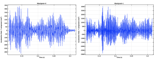
In the Settings window for 1D Plot Group, type Y Acceleration of Wheel (Frequency Spectrum) in the Label text field.
The gear rattle due to unloaded shaft causes initial transient vibration in the system. Remove this transient vibration data for the frequency spectrum plot.
3
Locate the Data section. From the Parameter selection (isMisaligned) list, choose First.
Point Graph 1
1
In the Model Builder window, expand the Y Acceleration of Wheel (Frequency Spectrum) node, then click Point Graph 1.
2
In the Settings window for Point Graph, locate the x-Axis Data section.
3
From the Parameter list, choose Discrete Fourier transform.
4
From the Show list, choose Frequency spectrum.
5
Select the Frequency range check box.
6
In the Maximum text field, type 2000.
7
Click to expand the Coloring and Style section. From the Width list, choose 2.
8
In the Y Acceleration of Wheel (Frequency Spectrum) toolbar, click  Plot.
Y Acceleration of Wheel (Frequency Spectrum)
1
In the Model Builder window, click Y Acceleration of Wheel (Frequency Spectrum).
2
In the Settings window for 1D Plot Group, locate the Data section.
3
From the Parameter selection (isMisaligned) list, choose Last.
4
In the Y Acceleration of Wheel (Frequency Spectrum) toolbar, click  Plot.
The rotor tilting in the bearing is compared in Figure 8 for aligned and misaligned cases. Follow the instructions below to reproduce this plot.
Rotor tilt at Bearing 2
1
In the Home toolbar, click  Add Plot Group and choose 1D Plot Group.
2
In the Settings window for 1D Plot Group, locate the Data section.
3
From the Dataset list, choose Study 1/Parametric Solutions 1 (2) (sol2).
4
In the Label text field, type Rotor tilt at Bearing 2.
5
Locate the Data section. From the Parameter selection (isMisaligned) list, choose First.
Global 1
1
Right-click Rotor tilt at Bearing 2 and choose Global.
2
In the Settings window for Global, locate the y-Axis Data section.
3
4
Locate the Coloring and Style section. From the Width list, choose 2.
5
Locate the Legends section. From the Legends list, choose Manual.
6
Rotor tilt at Bearing 2
1
In the Model Builder window, click Rotor tilt at Bearing 2.
2
In the Settings window for 1D Plot Group, locate the Plot Settings section.
3
Select the y-axis label check box. In the associated text field, type Rotor tilt (deg).
4
Locate the Title section. From the Title type list, choose Manual.
5
In the Title text area, type Misaligned=eval(isMisaligned).
6
In the Rotor tilt at Bearing 2 toolbar, click  Plot.
7
Locate the Data section. From the Parameter selection (isMisaligned) list, choose Last.
8
In the Rotor tilt at Bearing 2 toolbar, click  Plot.
Gear mesh contact force is an indicator of the rattling vibrations in shafts. This plot is shown in Figure 9, and it can be reproduced by using the instructions below.
Gear Mesh Contact Force
1
In the Home toolbar, click  Add Plot Group and choose 1D Plot Group.
2
In the Settings window for 1D Plot Group, locate the Data section.
3
From the Dataset list, choose Study 1/Parametric Solutions 1 (2) (sol2).
4
In the Label text field, type Gear Mesh Contact Force.
5
Locate the Data section. From the Parameter selection (isMisaligned) list, choose First.
Global 1
1
Right-click Gear Mesh Contact Force and choose Global.
2
In the Settings window for Global, click Replace Expression in the upper-right corner of the y-Axis Data section. From the menu, choose Component 1 (comp1)>Multibody Dynamics>Gear pairs>Gear Pair 1>mbd.grp1.Fc - Force at contact point - N.
3
Locate the Coloring and Style section. From the Width list, choose 2.
Gear Mesh Contact Force
1
In the Model Builder window, click Gear Mesh Contact Force.
2
In the Settings window for 1D Plot Group, locate the Title section.
3
From the Title type list, choose Manual.
4
In the Title text area, type Misaligned=eval(isMisaligned).
5
Locate the Legend section. Clear the Show legends check box.
6
In the Gear Mesh Contact Force toolbar, click  Plot.
7
Locate the Data section. From the Parameter selection (isMisaligned) list, choose Last.
8
In the Gear Mesh Contact Force toolbar, click  Plot.
Finally, use the instructions below to generate the animation of the stress variation in the shafts.
Animation 1
1
In the Results toolbar, click  Animation and choose Player.
2
In the Settings window for Animation, locate the Scene section.
3
From the Subject list, choose Stress (mbd).
4
Locate the Frames section. In the Number of frames text field, type 50.
5
Locate the Animation Editing section. From the Parameter value (isMisaligned) list, choose 1.
6
Click the  Play button in the Graphics toolbar.