PDF

Solar Dish Receiver
Introduction
A paraboloidal dish concentrator can focus incident solar radiation onto a target or cavity receiver, resulting in very high local heat fluxes. This can be used to generate steam, which can be used to power a generator, or hydrogen, which can be used directly as a fuel source. In some applications, such as hydrogen production via the solar thermal gasification of biomass in supercritical condition, the uniformity of the flux on the surface of the cavity receiver has a significant effect on the efficiency of hydrogen production (Ref. 1).
The basic concept behind the paraboloidal dish concentrator is shown in Figure 1. Solar radiation enters from the right and is reflected by the concentrator. The rays converge toward an extremely small area in the focal plane, where a cavity receiver can be positioned.
Figure 1: A simple solar concentrator system consisting of a parabolic dish and a small receiver. The color of the incident and focused rays corresponds to the ray intensity.
Of particular interest in evaluating the performance of solar collector-receiver systems is the concentration ratio, defined as the ratio of the incident flux to the ambient solar flux. A high concentration ratio usually means that the concentrator is capable of focusing solar radiation efficiently. When computing the concentration ratio, the incident flux can either be measured in the focal plane or on the surface of the cavity receiver.
A variety of computational methods to predict the concentration ratio are available. Shuai et al. (Ref. 1) compared the results of a Monte Carlo ray tracing code to compute the concentration ratios of several different cavity geometries. Jeter (Ref. 2) proposed a semi-analytical method in which the concentration ratio is computed via integration of the intensity distribution over the concentrator surface. A standard practice in many solar energy research institutions is to measure the concentrated solar flux using charge coupled device (CCD) imaging cameras (Ref. 3).
The ideal focusing system consists of a perfectly smooth paraboloidal dish that focuses collimated incident solar radiation onto a point in the focal plane that is infinitesimally small within the limit of the approximations of geometrical optics. However, several imperfections in this system cause the measured concentration ratio to deviate from the ideal case.
To accurately predict the concentration ratio, the finite size of the sun and the intensity distribution over the solar surface must be considered. The intensity profile on the solar disk is referred to as sunshape. Solar intensity is greatest at the center of the solar disk and decreases closer to the periphery of the disk, a phenomenon called solar limb darkening.
Integration Method for Ideally Smooth Solar Collectors
A method for computing the concentration ratio in the focal plane in the absence of surface roughness is described by Jeter (Ref. 2). Consider differential area elements on the surface of the concentrator at rc and on the focal plane of the receiver at r, as shown in Figure 2.
Figure 2: Diagram of the paraboloidal solar concentrator.
where the surface normals at the concentrator and focal plane are and , respectively, and O is the focus. The following angles are defined:
The concentration ratio at r is
(1)
(2)
where:
f (SI unit: W/(m2 steradian)) is the radiant intensity
Ω denotes surface integration over the collector surface
I0 (SI unit: W/m2) is the incident solar flux
ψm is the maximum solar disk angle
dAc (SI unit: m2) is a differential area element on the surface of the collector
In Equation 2 it is assumed that the incident solar flux does not vary as a function of position on the solar disk; that is, no solar limb darkening is considered. However, it would be possible to extend Equation 2 to account for solar limb darkening by including a term dependent on the angle δ on the right-hand side.
In this model, Equation 1 is implemented using the dest() operator. The dest() operator evaluates a term in a nonlocal integration coupling on the destination side. For example, including the term u/((dest(x)-x)^2+(dest(y)-y)^2) in a nonlocal integration coupling gives the following function of x and y:
Model Definition
A parabolic solar dish concentrator with a focal length, f, of m is constructed using a built-in Part from the Part Library for the Ray Optics Module. The geometry also includes a small cylinder, one surface of which lies in the focal plane. The incident flux on this surface will be computed, then used to compute the concentration ratio. By adjusting the shape of the cylinder it would be possible to compute the concentration ratios for various cavity geometries, as in Ref. 1, but for the present analysis, only the concentration ratio in the focal plane is computed.
If the dish was a perfect reflector (all of the incoming radiation reflected specularly), the dish was perfectly smooth, and the rays from the sun behaved as planar wavefronts from an infinitely distant point source, all of the incoming rays would be focused on a single point on the collector, at the focus of the paraboloid (within the limits of the geometrical optics approximation). However, in this model, several deviations from this idealized case are considered.
A dedicated boundary condition called Illuminated Surface is used to release rays directly from the surface of the dish, initializing their directions as if they were reflected from a distant plane wave source. The direction at which the rays are released from the surface of the dish depends on the incoming ray direction vector ni and the outward surface normal ns, according to the formula
(3)
The intensity of each individual ray can be computed along its trajectory; the evolution of ray intensity depends heavily on the curvature of the dish. More details on intensity computation can be found in the Ray Optics Module User’s Guide.
Each ray released is also assigned a fixed power, which is assigned an appropriate value based on the Source power setting for the Illuminated Surface feature. When the rays reach the surface of the solar collector, they are stopped by the Wall feature. The Deposited Ray Power subfeature computes the incident heat flux in the focal plane. By taking the ratio of the deposited flux to the incoming solar flux, the concentration ratio on the surface can be computed.
Some of the incoming radiation is absorbed by the dish itself. Even a newly installed dish absorbs a significant fraction of the incident radiation, and parts of the dish can degrade over the course of its lifetime, reducing its efficiency (Ref. 3). In this model, the absorption coefficient is set to 0.1, meaning that 90% of the incoming radiation is reflected.
An additional correction is included due to the finite size of the sun. Not all incident rays will be parallel; instead, the incident rays are sampled from a narrow cone with maximum angle, ψm, of 4.65 mrad. In practice, some radiation is also emitted from the circumsolar region surrounding the solar disk, instead of the solar disk itself, but this radiation is neglected in the present model; that is, a circumsolar ratio (CSR) of zero is assumed. When rays are released from points other than the center of the solar dish, their initial intensity can be reduced to account for solar limb darkening effects.
Since the surface of the dish is not perfectly smooth, the reflected rays are not all released at the exact direction given by Equation 3. Instead, the surface normal is perturbed by an additional angle that is sampled from a Rayleigh distribution:
where (SI unit: rad) is the surface slope error1.
The model includes two studies, each corresponding to a separate instance of the Illuminated Surface feature. For each study, rays are released from 100,000 distinct points. At each point, the incident ray direction is perturbed by a random angle; the probability density of these perturbations is uniform within a cone of angle ψs.
For the first study, no limb darkening model is used and the surface is assumed to be perfectly smooth and reflective. The resulting concentration ratio is compared to the semi-analytical method of Jeter (Ref. 2).
For the second study, a limb darkening model is used to reduce the intensity of solar radiation emitted from the edge of the solar dish. The built-in limb darkening model follows an exponential fit, with wavelength-dependent exponents as described in Ref. 5. The resulting concentration ratio in the focal plane is compared to results in Ref. 1.
For each study, the concentration ratio is computed on a small circular disc, centered at the origin, which lies in the focal plane.
Simply plotting the concentration ratio as a function of the radial distance and azimuthal angle in the focal plane is not sufficient to compare against the data of Refs. 1-2 because there is a significant amount of statistical noise in the model. This is due to the random nature of the incident ray direction vectors at each release point. To smooth some of this statistical noise, the average concentration ratio is taken over all azimuthal angles for each value of the radial coordinate in the focal plane:
(4)
Equation 4 is implemented using a General Projection nonlocal coupling. A General Projection nonlocal coupling evaluates a series of line or curve integrals on a source. In this example, the General Projection 1 node integrates the accumulated variable over concentric circles in the focal plane, centered at the origin.
Results and Discussion
The ray trajectories emanating from the solar dish can be seen in Figure 3. Almost every ray is stopped by the receiver, with only an extremely small number of propagating rays visible above the focal plane.
Figure 3: The ray trajectories emanate from the illuminated surface and hit the receiver.
The incident heat flux arriving on the surface of the collector is shown in Figure 4. The heat flux is extremely high, with an average value of about 23 W/mm2 near the center of the focal plane. The statistical noise is also apparent, since in some boundary mesh elements the incident heat flux exceeds 30 W/mm2. If smoothing is disabled in the plot, then in a very small number of boundary elements the incident flux is shown to be even greater, as high as 51 W/mm2. This demonstrates the need for averaging in the azimuthal direction to more consistently compare the concentration ratio to published values.
The azimuthally averaged concentration ratio is plotted in Figure 5 along with the semi-analytical solution of Jeter (Ref. 2). The data are shown to be in close agreement.
Figure 4: Incident heat flux on the surface of the receiver, resulting from an ideally smooth, non-absorbing paraboloidal reflector. Solar limb darkening effects have also been neglected.
Figure 5: Comparison of the azimuthally averaged, computed concentration ratio in the focal plane to a semi-analytical solution. The two solutions are in close agreement.
The ray trajectories resulting from the second study are shown in Figure 6. Compared to Figure 3, a substantial number of rays now miss the receiver and continue to propagate, reducing the efficiency of the cavity receiver.
Figure 6: Reflection of solar radiation by a paraboloidal dish. Surface roughness, absorption, and solar limb darkening have all been taken into account.
The flux distribution in the focal plane is shown in Figure 7. Compared to Figure 4, the distribution is much more widespread, lacking any well-defined plateau. The maximum flux has also been considerably reduced.
The comparison of the azimuthally averaged concentration ratio to Ref. 1 is shown in Figure 8. The two solutions are again shown to be in close agreement. Further statistical convergence could be achieved by increasing the number of rays and refining the mesh on the focal plane, at the cost of increased memory usage and solution time.
Finally, the incident heat flux distributions from the two studies are directly compared in Figure 9.
Figure 7: Flux distribution in the focal plane when taking surface roughness, absorption, and solar limb darkening into account.
Figure 8: Comparison of the azimuthally averaged concentration ratio to published data.
Figure 9: Direct comparison of the flux distributions when including roughness, absorption, and solar limb darkening (the “Real Collector”), and when neglecting these effects (the “Ideal Collector”).
References
1. Y. Shuai, X-L. Xia, and H-P. Tan, “Radiation performance of dish solar concentrator/cavity receiver systems,” Sol. Energy, vol. 82, pp. 13–21, 2008.
2. S.M. Jeter, “The distribution of concentrated solar radiation in paraboloidal collectors”, J. Sol. Energy Eng., vol. 108, pp. 219–225, 1986.
3. G. Johnston, “Focal region measurements of the 20 m2 tiled dish at the Australian national university,” Sol. Energy, vol. 63, no. 2, pp. 117–124, 1998.
4. M. Schubnell, “Sunshape and its influence on the flux distribution in imaging solar concentrators,” J. Sol. Energy Eng., vol. 114, pp. 260–266, 1992.
5. D. Hestroffer and C. Magnan, “Wavelength dependency of the Solar limb darkening,” Astron. Astrophys., vol. 333, pp. 338–342, 1998.
Application Library path: Ray_Optics_Module/Solar_Radiation/solar_dish_receiver
Modeling Instructions
From the File menu, choose New.
New
In the New window, click  Model Wizard.
Model Wizard
1
In the Model Wizard window, click  3D.
2
In the Select Physics tree, select Optics>Ray Optics>Geometrical Optics (gop).
3
Click Add.
4
Click  Study.
5
In the Select Study tree, select Preset Studies for Selected Physics Interfaces>Ray Tracing.
6
Geometry 1
Define some parameters for the geometry setup.
Global Definitions
Parameters 1
1
In the Model Builder window, under Global Definitions click Parameters 1.
2
In the Settings window for Parameters, locate the Parameters section.
3
Geometry 1
Cylinder 1 (cyl1)
1
In the Geometry toolbar, click  Cylinder.
2
In the Settings window for Cylinder, locate the Size and Shape section.
3
In the Radius text field, type 30[mm].
4
In the Height text field, type 100[mm].
5
Click  Build All Objects.
Part Libraries
1
In the Geometry toolbar, click  Parts and choose Part Libraries.
2
In the Model Builder window, click Geometry 1.
3
In the Part Libraries window, select Ray Optics Module>3D>Mirrors>paraboloidal_reflector_shell_3d in the tree.
4
Click  Add to Geometry.
5
In the Select Part Variant dialog box, select Specify rim angle in the Select part variant list.
6
Geometry 1
Paraboloidal Reflector Shell 3D 1 (pi1)
1
In the Model Builder window, under Component 1 (comp1)>Geometry 1 click Paraboloidal Reflector Shell 3D 1 (pi1).
2
In the Settings window for Part Instance, locate the Input Parameters section.
3
4
Locate the Position and Orientation of Output section. Find the Displacement subsection. In the zw text field, type -f.
5
Click to expand the Boundary Selections section. In the table, select the Keep check box for All.
Global Definitions
In the Model Builder window, collapse the Global Definitions node.
Geometry 1
In the Model Builder window, collapse the Component 1 (comp1)>Geometry 1 node.
Definitions
Integration 1 (intop1)
1
In the Definitions toolbar, click  Nonlocal Couplings and choose Integration.
2
In the Settings window for Integration, locate the Source Selection section.
3
From the Geometric entity level list, choose Boundary.
4
From the Selection list, choose All (Paraboloidal Reflector Shell 3D 1).
Interpolation 1 (int1)
1
In the Definitions toolbar, click  Interpolation.
Load the expected solution data from Ref. 1.
2
In the Settings window for Interpolation, locate the Definition section.
3
From the Data source list, choose File.
4
Click  Browse.
5
6
Click  Import.
7
Locate the Units section. In the Argument table, enter the following settings:
8
In the Function table, enter the following settings:
Add a selection for the surface of the paraboloidal dish, where the reflected rays are released.
Focal Plane
1
In the Definitions toolbar, click  Explicit.
2
In the Settings window for Explicit, type Focal Plane in the Label text field.
3
Locate the Input Entities section. From the Geometric entity level list, choose Boundary.
4
Variables 1
1
In the Model Builder window, right-click Definitions and choose Variables.
Define variables to compute the concentration ratio for an ideal parabolic solar concentrator, following Jeter (Ref. 2). To save time, these variables can be loaded from a file.
2
In the Settings window for Variables, locate the Variables section.
3
Click  Load from File.
4
General Projection 1 (genproj1)
1
In the Definitions toolbar, click  Nonlocal Couplings and choose General Projection.
2
In the Settings window for General Projection, locate the Source Selection section.
3
From the Geometric entity level list, choose Boundary.
4
From the Selection list, choose Focal Plane.
5
Click the  Go to Default View button in the Graphics toolbar.
6
Locate the Source Map section. In the x-expression text field, type r.
7
In the y-expression text field, type theta.
8
Locate the Destination Map section. In the x-expression text field, type r.
9
In the Model Builder window, collapse the Definitions node.
Geometrical Optics (gop)
1
In the Model Builder window, under Component 1 (comp1) click Geometrical Optics (gop).
2
In the Settings window for Geometrical Optics, locate the Domain Selection section.
3
Click  Clear Selection.
4
Locate the Intensity Computation section. From the Intensity computation list, choose Compute power.
5
Locate the Ray Release and Propagation section. In the Maximum number of secondary rays text field, type 0.
Add two instances of the Illuminated Surface release feature. One of these features will include surface roughness and solar limb darkening. One release feature will be used in each of the two studies in this model.
Ideal Illuminated Surface
1
In the Physics toolbar, click  Boundaries and choose Illuminated Surface.
2
In the Settings window for Illuminated Surface, type Ideal Illuminated Surface in the Label text field.
3
Locate the Boundary Selection section. From the Selection list, choose All (Paraboloidal Reflector Shell 3D 1).
4
Locate the Initial Position section. From the Initial position list, choose Density.
5
In the N text field, type 100000.
6
Locate the Ray Direction Vector section. Specify the Li vector as
7
Locate the Angular Perturbations section. From the Corrections for finite source diameter list, choose Sample from conical distribution.
8
Locate the Total Source Power section. In the Psrc text field, type A*I0.
9
Locate the Angular Perturbations section. In the ψm text field, type psim.
Real Illuminated Surface
1
In the Physics toolbar, click  Boundaries and choose Illuminated Surface.
2
In the Settings window for Illuminated Surface, type Real Illuminated Surface in the Label text field.
3
Locate the Boundary Selection section. From the Selection list, choose All (Paraboloidal Reflector Shell 3D 1).
4
Locate the Initial Position section. From the Initial position list, choose Density.
5
In the N text field, type 100000.
6
Locate the Ray Direction Vector section. Specify the Li vector as
7
In the α text field, type 0.1.
8
Locate the Angular Perturbations section. From the Corrections for finite source diameter list, choose Sample from conical distribution.
9
In the ψm text field, type psim.
10
From the Limb darkening model list, choose Empirical power law.
11
Select the Include surface roughness check box.
12
In the σ text field, type sig.
13
Locate the Total Source Power section. In the Psrc text field, type A*I0.
14
Locate the Incident Ray Polarization section. From the Initial polarization type list, choose Unpolarized.
Focal Plane
1
In the Physics toolbar, click  Boundaries and choose Wall.
2
In the Settings window for Wall, type Focal Plane in the Label text field.
3
Locate the Boundary Selection section. From the Selection list, choose Focal Plane.
4
Click the  Go to Default View button in the Graphics toolbar.
Use the Deposited Ray Power node to compute the incident heat flux in the focal plane.
Deposited Ray Power 1
1
In the Physics toolbar, click  Attributes and choose Deposited Ray Power.
2
In the Model Builder window, collapse the Geometrical Optics (gop) node.
Mesh 1
1
In the Model Builder window, under Component 1 (comp1) click Mesh 1.
2
In the Settings window for Mesh, locate the Physics-Controlled Mesh section.
3
From the Element size list, choose Extremely fine.
4
Locate the Sequence Type section. From the list, choose User-controlled mesh.
Size 1
1
In the Model Builder window, right-click Free Triangular 1 and choose Size.
2
In the Settings window for Size, locate the Geometric Entity Selection section.
3
Click  Clear Selection.
4
5
Locate the Element Size section. Click the Custom button.
Use an extremely fine mesh on the focal plane to improve the resolution of the deposited ray power.
6
Locate the Element Size Parameters section.
7
Select the Maximum element size check box. In the associated text field, type 5E-4.
8
Select the Minimum element size check box. In the associated text field, type 2E-4.
9
In the Model Builder window, collapse the Mesh 1 node.
10
In the Model Builder window, right-click Mesh 1 and choose Build All.
Study 1
Step 1: Ray Tracing
1
In the Model Builder window, under Study 1 click Step 1: Ray Tracing.
2
In the Settings window for Ray Tracing, locate the Study Settings section.
3
From the Time-step specification list, choose Specify maximum path length.
4
In the Lengths text field, type 0 4.
5
Locate the Physics and Variables Selection section. Select the Modify model configuration for study step check box.
6
In the tree, select Component 1 (comp1)>Geometrical Optics (gop)>Real Illuminated Surface.
7
Solution 1 (sol1)
1
In the Study toolbar, click  Show Default Solver.
Specify a manual time step size to speed up the computation and reduce the file size.
2
In the Model Builder window, expand the Solution 1 (sol1) node, then click Time-Dependent Solver 1.
3
In the Settings window for Time-Dependent Solver, click to expand the Time Stepping section.
4
From the Steps taken by solver list, choose Manual.
5
In the Time step text field, type 4[m]/c_const.
6
In the Model Builder window, collapse the Study 1 node.
7
In the Study toolbar, click  Compute.
Results
Ray Trajectories, Ideal Reflector
1
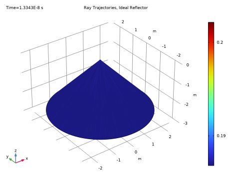
In the Settings window for 3D Plot Group, type Ray Trajectories, Ideal Reflector in the Label text field.
2
Click to expand the Title section. From the Title type list, choose Manual.
3
In the Title text area, type Ray Trajectories, Ideal Reflector.
4
In the Model Builder window, expand the Ray Trajectories, Ideal Reflector node.
Color Expression 1
1
In the Model Builder window, expand the Results>Ray Trajectories, Ideal Reflector>Ray Trajectories 1 node, then click Color Expression 1.
2
In the Settings window for Color Expression, click Replace Expression in the upper-right corner of the Expression section. From the menu, choose Component 1 (comp1)>Geometrical Optics>Intensity and polarization>gop.Q - Ray power - W.
3
In the Ray Trajectories, Ideal Reflector toolbar, click  Plot.
4
Click the  Zoom Extents button in the Graphics toolbar. Compare the resulting plot with Figure 3.
Ray Trajectories, Ideal Reflector
In the Model Builder window, collapse the Results>Ray Trajectories, Ideal Reflector node.
Surface 1
1
In the Results toolbar, click  More Datasets and choose Surface.
2
In the Settings window for Surface, locate the Parameterization section.
3
From the x- and y-axes list, choose XY-plane.
4
Locate the Selection section. From the Selection list, choose Focal Plane.
5
Click the  Go to Default View button in the Graphics toolbar.
Deposited Power, Ideal Reflector
1
In the Results toolbar, click  2D Plot Group.
2
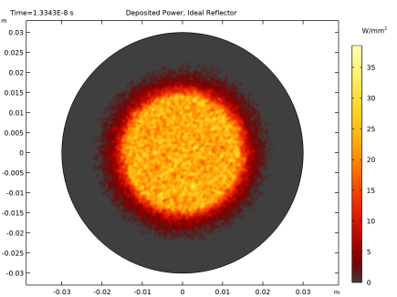
In the Settings window for 2D Plot Group, type Deposited Power, Ideal Reflector in the Label text field.
3
Click to expand the Title section. From the Title type list, choose Manual.
4
In the Title text area, type Deposited Power, Ideal Reflector.
5
Locate the Data section. From the Dataset list, choose Surface 1.
6
Locate the Color Legend section. Select the Show units check box.
Surface 1
1
Right-click Deposited Power, Ideal Reflector and choose Surface.
2
In the Settings window for Surface, click Replace Expression in the upper-right corner of the Expression section. From the menu, choose Component 1 (comp1)>Geometrical Optics>Accumulated variables>Boundary heat source comp1.gop.wall1.bsrc1.Qp>gop.wall1.bsrc1.Qp - Boundary heat source - W/m².
3
Locate the Expression section. In the Unit field, type W/mm^2.
4
Locate the Coloring and Style section. Click  Change Color Table.
5
In the Color Table dialog box, select Thermal>GrayBody in the tree.
6
7
In the Settings window for Surface, click to expand the Quality section.
8
From the Resolution list, choose No refinement.
9
In the Deposited Power, Ideal Reflector toolbar, click  Plot.
10
Click the  Zoom Extents button in the Graphics toolbar. Compare the resulting plot with Figure 4.
Cut Line 3D 1
1
In the Results toolbar, click  Cut Line 3D.
2
In the Settings window for Cut Line 3D, locate the Line Data section.
3
In row Point 1, set X to 1E-4.
4
In row Point 2, set X to 0.03-1E-4.
5
From the Snapping list, choose Snap to closest boundary.
Concentration Ratios, Ideal Reflector
1
In the Results toolbar, click  1D Plot Group.
2
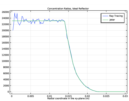
In the Settings window for 1D Plot Group, type Concentration Ratios, Ideal Reflector in the Label text field.
3
Click to expand the Title section. From the Title type list, choose Manual.
4
In the Title text area, type Concentration Ratios, Ideal Reflector.
5
Locate the Data section. From the Dataset list, choose Cut Line 3D 1.
6
From the Time selection list, choose Last.
Line Graph 1
1
Right-click Concentration Ratios, Ideal Reflector and choose Line Graph.
Plot the azimuthally averaged, smoothed heat source on the cylinder using the nonlocal projection coupling previously defined.
2
In the Settings window for Line Graph, locate the y-Axis Data section.
3
In the Expression text field, type genproj1(gop.wall1.bsrc1.Qp)/genproj1(I0).
4
Click to expand the Quality section. From the Resolution list, choose No refinement.
5
Locate the x-Axis Data section. From the Parameter list, choose Expression.
6
In the Expression text field, type r.
7
Click to expand the Legends section. Select the Show legends check box.
8
From the Legends list, choose Manual.
9
10
In the Concentration Ratios, Ideal Reflector toolbar, click  Plot.
Line Graph 2
1
Right-click Line Graph 1 and choose Duplicate.
2
In the Settings window for Line Graph, locate the y-Axis Data section.
3
In the Expression text field, type cr.
4
Click to expand the Title section. From the Title type list, choose None.
5
Locate the Legends section. In the table, enter the following settings:
6
In the Concentration Ratios, Ideal Reflector toolbar, click  Plot. Compare the resulting plot with Figure 5. This figure shows the radial variation in the idealized concentration ratio. Now create a second study in which roughness, absorption, and limb darkening effects are considered.
Add Study
1
In the Home toolbar, click  Add Study to open the Add Study window.
2
Go to the Add Study window.
3
Find the Studies subsection. In the Select Study tree, select Preset Studies for Selected Physics Interfaces>Ray Tracing.
4
Click Add Study in the window toolbar.
5
In the Home toolbar, click  Add Study to close the Add Study window.
Study 2
Step 1: Ray Tracing
1
In the Settings window for Ray Tracing, locate the Study Settings section.
2
From the Time-step specification list, choose Specify maximum path length.
3
In the Lengths text field, type 0 4.
4
Locate the Physics and Variables Selection section. Select the Modify model configuration for study step check box.
5
In the tree, select Component 1 (comp1)>Geometrical Optics (gop)>Ideal Illuminated Surface.
6
Solution 2 (sol2)
1
In the Study toolbar, click  Show Default Solver.
Specify a manual time step size to speed up the computation and reduce the file size.
2
In the Model Builder window, expand the Solution 2 (sol2) node, then click Time-Dependent Solver 1.
3
In the Settings window for Time-Dependent Solver, locate the Time Stepping section.
4
From the Steps taken by solver list, choose Manual.
5
In the Time step text field, type 4[m]/c_const.
6
In the Model Builder window, collapse the Study 2 node.
7
In the Study toolbar, click  Compute.
Results
Ray Trajectories, Real Reflector
1
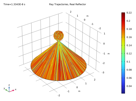
In the Settings window for 3D Plot Group, type Ray Trajectories, Real Reflector in the Label text field.
2
Locate the Title section. From the Title type list, choose Manual.
3
In the Title text area, type Ray Trajectories, Real Reflector.
4
In the Model Builder window, expand the Ray Trajectories, Real Reflector node.
Color Expression 1
1
In the Model Builder window, expand the Results>Ray Trajectories, Real Reflector>Ray Trajectories 1 node, then click Color Expression 1.
2
In the Settings window for Color Expression, locate the Expression section.
3
In the Expression text field, type gop.Q.
4
In the Ray Trajectories, Real Reflector toolbar, click  Plot.
5
Click the  Go to Default View button in the Graphics toolbar. Compare the resulting plot with Figure 6.
Ray Trajectories, Real Reflector
In the Model Builder window, collapse the Results>Ray Trajectories, Real Reflector node.
Surface 1
Create duplicates of the Surface and Cut Line 3D datasets that point to Solution 2.
Surface 2
1
In the Model Builder window, under Results>Datasets right-click Surface 1 and choose Duplicate.
2
In the Settings window for Surface, locate the Data section.
3
From the Dataset list, choose Study 2/Solution 2 (sol2).
Cut Line 3D 2
1
In the Model Builder window, under Results>Datasets right-click Cut Line 3D 1 and choose Duplicate.
2
In the Settings window for Cut Line 3D, locate the Data section.
3
From the Dataset list, choose Study 2/Solution 2 (sol2).
Deposited Power, Real Reflector
1
In the Model Builder window, right-click Deposited Power, Ideal Reflector and choose Duplicate.
2
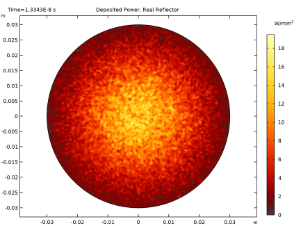
In the Settings window for 2D Plot Group, type Deposited Power, Real Reflector in the Label text field.
3
Locate the Title section. In the Title text area, type Deposited Power, Real Reflector.
4
Locate the Data section. From the Dataset list, choose Surface 2.
5
In the Deposited Power, Real Reflector toolbar, click  Plot.
6
Click the  Zoom Extents button in the Graphics toolbar. Compare the resulting plot with Figure 7.
Concentration Ratios, Real Reflector
1
In the Model Builder window, right-click Concentration Ratios, Ideal Reflector and choose Duplicate.
2
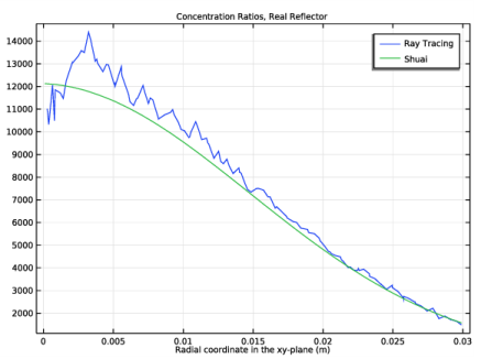
In the Settings window for 1D Plot Group, type Concentration Ratios, Real Reflector in the Label text field.
3
Locate the Title section. In the Title text area, type Concentration Ratios, Real Reflector.
4
Locate the Data section. From the Dataset list, choose Cut Line 3D 2.
Line Graph 1
1
In the Model Builder window, expand the Concentration Ratios, Real Reflector node, then click Line Graph 1.
2
In the Settings window for Line Graph, locate the Legends section.
3
Line Graph 2
1
In the Model Builder window, click Line Graph 2.
2
In the Settings window for Line Graph, locate the y-Axis Data section.
3
In the Expression text field, type int1(r)/I0.
4
Locate the Legends section. In the table, enter the following settings:
5
In the Concentration Ratios, Real Reflector toolbar, click  Plot. Compare the resulting plot with Figure 8.
Create another plot group to directly compare the flux distributions in the focal plane for the two solutions.
Deposited Power, Real and Ideal Reflectors
1
In the Model Builder window, right-click Deposited Power, Ideal Reflector and choose Duplicate.
2
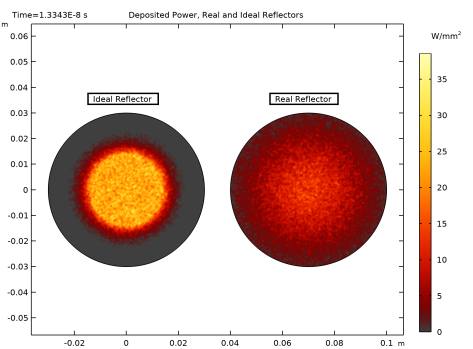
In the Settings window for 2D Plot Group, type Deposited Power, Real and Ideal Reflectors in the Label text field.
3
Locate the Title section. In the Title text area, type Deposited Power, Real and Ideal Reflectors.
Surface 1
1
In the Model Builder window, expand the Results>Deposited Power, Real Reflector node.
2
Right-click Surface 1 and choose Copy.
Surface 2
1
In the Model Builder window, expand the Results>Deposited Power, Real and Ideal Reflectors node.
2
Right-click Deposited Power, Real and Ideal Reflectors and choose Paste Surface.
3
In the Settings window for Surface, locate the Data section.
4
From the Dataset list, choose Surface 2.
5
Click to expand the Inherit Style section. From the Plot list, choose Surface 1.
Translation 1
1
Right-click Surface 2 and choose Translation.
2
In the Settings window for Translation, locate the Translation section.
3
In the x text field, type 0.07[m].
4
In the Deposited Power, Real and Ideal Reflectors toolbar, click  Plot.
Deposited Power, Real and Ideal Reflectors
Create two Annotation features to identify the two plots in the Graphics window.
Annotation 1
1
In the Model Builder window, right-click Deposited Power, Real and Ideal Reflectors and choose Annotation.
2
In the Settings window for Annotation, locate the Annotation section.
3
In the Text text field, type Ideal Reflector.
Enter the coordinates for the annotations. The exact coordinates may vary depending on the aspect ratio of the Graphics window.
4
Locate the Position section. In the x text field, type -0.015.
5
In the y text field, type 0.038.
6
Locate the Coloring and Style section. Clear the Show point check box.
7
Select the Show frame check box.
Annotation 2
1
Right-click Deposited Power, Real and Ideal Reflectors and choose Annotation.
2
In the Settings window for Annotation, locate the Annotation section.
3
In the Text text field, type Real Reflector.
4
Locate the Position section. In the x text field, type 0.055.
5
In the y text field, type 0.038.
6
Locate the Coloring and Style section. Clear the Show point check box.
7
Select the Show frame check box.
8
In the Deposited Power, Real and Ideal Reflectors toolbar, click  Plot.
9
Click the  Zoom Extents button in the Graphics toolbar. Compare the resulting plot with Figure 9.
 

1
The definition of the surface slope error used in the Illuminated Surface feature seems to differ from the definition used by Shuai et al. For the Illuminated Surface, the surface slope error is used to perturb the surface normal direction, not the incident ray direction. As a result, values of the surface slope error used in this model differ from the corresponding results in Ref.1 by a factor of 2.